import random
import pandas as pd
random.seed(2611121)
n_realizations=4000PP5000 problem set 1: univariate-stats
Choose one of the following 3 options
Solve exercise 2611121 and exercise 10812121614
Solve exercise 16610101020
Solve exercise 1200110030
Items marked OPTIONAL are extensions, you can skip them and still receive full credit.
The deadline is Tuesday, September 01, 19:30.
You are allowed to discuss exercises and to collaborate, but this is an individual assignment.
Upload a pdf document with your answers. Add brief comments, particularly if you reviewed your answers and found them suspicious or implausible. Don’t overthink formatting and cosmetics: copy-pasting console output or taking screenshots is fine for this assignment.
ImportantLesson learned
While this assignment was unusual, and the optional uploads may have given the wrong idea, I should have been clearer that you produce results, not code, and you provide code to reproduce your results, not to produce them.
Acknowledge any assistance received, whether from humans or from AIs.
Alongside your pdf answers, but separate from them, you must provide replication code sufficient to produce every result, table, plot… in your pdf answers.
Exercise 2611121: comparing 2d6+1 and 1d12+1
Start your code with:
Generate n_realizations realizations of:
2d6+1, i.e. the result of rolling two d6, adding the faces, and adding 1
and n_realizations realizations of:
1d12+1, i.e. the result of rolling 1 d12, and adding 1
Store the results in lists named respectively: realizations_2d6_plus_1 and realizations_1d12_plus_1
Put both lists in the same pandas dataframe.
Produce a table with 2 columns named 2d6_plus_1 and 1d12_plus_1 and rows displaying:
minimum
maximum
mean
variance
as well as 5 rows for the frequency of:
realization >= 8
realization >= 9
realization >= 10
realization >= 11
realization >= 12
import random
import pandas as pd
random.seed(2611121)
n_realizations=4000

realizations_2d6_plus_1 = [
    random.randint(1, 6) + random.randint(1, 6) + 1
    for i in range(n_realizations)
]

realizations_1d12_plus_1 = [
    random.randint(1, 12) + 1
    for i in range(n_realizations)
]

df = pd.DataFrame({
    "2d6_plus_1": realizations_2d6_plus_1,
    "1d12_plus_1": realizations_1d12_plus_1
})
print(df)

results_df = df.describe()
### Using .describe() to produce min, max, mean and std
results_df.loc["variance"] = results_df.loc["std"] ** 2
### std is the sqrt of variance, so we need to square std to recover variance.
## dataframes routinely allow operations applying to a whole row
## The .loc method df.loc[row_selector, column_selector]
## selects either a row or a column or a cell (if you specify both row and column)
## .iloc selects using integer positions

print(results_df)
results_df = results_df.drop(
    ["count", "std", "25%", "50%", "75%"]
)
## dropping the rows we do not need

for threshold in range(8, 13):

    results_df.loc[f"frequency >= {threshold}"] = [
        (df["2d6_plus_1"] >= threshold).sum() / n_realizations,
        (df["1d12_plus_1"] >= threshold).sum() / n_realizations
    ]

## each ">= threshold" comparison creates a Boolean data Series
## e.g. (df["2d6_plus_1"] >= 11) is a data Series with Name: 2d6_plus_1, Length: 4000, dtype: bool
## dtype: bool, Boolean meaning that values are either True or False
## .sum() counts each "True" as 1 and each "False" as 0, so it counts True values,
## dividing by n_realizations converts the count into a frequency.
## finally, results_df.loc[f"frequency >= {threshold}"] = [a,b]
## means "we add a row to the dataframe results_df
###... called "frequency >= {threshold}"
###... and the values of the new row will be [a,b]

print(results_df.round(4))
2d6_plus_1 1d12_plus_1
0 8 8
1 5 7
2 12 11
3 7 3
4 4 9
... ... ...
3995 8 8
3996 7 9
3997 6 2
3998 10 4
3999 12 10
[4000 rows x 2 columns]
2d6_plus_1 1d12_plus_1
count 4000.000000 4000.000000
mean 8.034750 7.424500
std 2.439473 3.482575
min 3.000000 2.000000
25% 6.000000 4.000000
50% 8.000000 7.000000
75% 10.000000 10.000000
max 13.000000 13.000000
variance 5.951030 12.128332
2d6_plus_1 1d12_plus_1
mean 8.0348 7.4245
min 3.0000 2.0000
max 13.0000 13.0000
variance 5.9510 12.1283
frequency >= 8 0.5890 0.4878
frequency >= 9 0.4198 0.4068
frequency >= 10 0.2838 0.3298
frequency >= 11 0.1725 0.2488
frequency >= 12 0.0888 0.167210812121614 Hypothesis testing — Reverse the hypotheses
The goal of this exercise is to follow the lecture notes’ example of hypothesis testing, except we flip the hypotheses. The null hypothesis is now H0: the d6 is rigged, and the alternative hypothesis is now H1: the d6 is fair. The test statistic is the sample mean.
Start your code with:
import random
random.seed(10812121614)

n_simulations = 2000
alpha = 0.10
sample_size = 50

interval_widths_fair = [12, 12, 12, 12, 12, 12]
interval_widths_rigged = [10, 8, 12, 12, 16, 14]

def jitter(x, scale):
    return x + random.uniform(-scale, scale)
Apply a small jitter (1e-6) whenever you compute a test statistic. The jitter ensures that no two samples have exactly the same value of the test statistic.
Distribution of the test statistic and decision rule.
Draw
n_simulationssamples assuming H0 and compute the test statistic for each sample.Display the distribution of the test statistic under H0 as a histogram.
Draw
n_simulationssamples assuming H1 and compute the test statistic for each sample.Display the distribution of the test statistic under H1 as a histogram on the same graph.
Choose the decision rule (the rejection region) such that when H0 is true, type I errors occur with probability
alpha.
30 trials of testing a d6 of unknown type.
Perform 30 trials: in each trial, the type of d6 is chosen randomly (chosen to be fair or rigged with equal probability), then a sample of size sample_size is generated, the test statistic is computed, then a decision to reject or not the null hypothesis is taken. For each trial, print:
true type of the d6
realization of the test statistic in this sample
p-value of the realization of the test statistic assuming H0 is true
Decision (either
reject H0orfail to reject H0)Whether the decision was correct, a type I error, or a type II error
From trials to simulations
Using the samples drawn previously, compute the frequency of type I errors.
Using the samples drawn previously, compute the frequency of type II errors.
Give the empirical power of the test.
ImportantLesson learned
I should have been clearer that you should re-use the n_simulations samples rather than the 30 trials. Estimating power on the subset of 30 trials where d6 was fair is far from precise, and the frequency of type I errors should be exactly 0.1, which should be a good sanity check.
import random
import matplotlib.pyplot as plt

random.seed(10812121614)

n_simulations = 2000
alpha = 0.10
sample_size = 50

interval_widths_fair = [12, 12, 12, 12, 12, 12]
interval_widths_rigged = [10, 8, 12, 12, 16, 14]

def jitter(x, scale):
    return x + random.uniform(-scale, scale)


#%% Construct the fair and rigged d6

assert sum(interval_widths_fair) == 72
assert sum(interval_widths_rigged) == 72


thresholds_fair = []
running_total = 0

for interval_width in interval_widths_fair:
    running_total += interval_width
    thresholds_fair.append(running_total)


thresholds_rigged = []
running_total = 0

for interval_width in interval_widths_rigged:
    running_total += interval_width
    thresholds_rigged.append(running_total)


def roll_fair_d6():

    draw = random.randint(1, 72)

    for face, threshold in enumerate(thresholds_fair, start=1):
        if draw <= threshold:
            return face


def roll_rigged_d6():

    draw = random.randint(1, 72)

    for face, threshold in enumerate(thresholds_rigged, start=1):
        if draw <= threshold:
            return face


#%% Distribution of the test statistic under H0 and H1

# H0: the d6 is rigged
# H1: the d6 is fair

test_statistics_H0 = []
test_statistics_H1 = []

for i_simulation in range(n_simulations):

    sample_H0 = []

    for i_roll in range(sample_size):
        sample_H0.append(roll_rigged_d6())

    test_statistic_H0 = sum(sample_H0) / sample_size
    test_statistic_H0 = jitter(test_statistic_H0, 1e-6)

    test_statistics_H0.append(test_statistic_H0)


    sample_H1 = []

    for i_roll in range(sample_size):
        sample_H1.append(roll_fair_d6())

    test_statistic_H1 = sum(sample_H1) / sample_size
    test_statistic_H1 = jitter(test_statistic_H1, 1e-6)

    test_statistics_H1.append(test_statistic_H1)


# Because fair d6 samples tend to have lower sample means,
# the rejection region is in the lower tail.

sorted_test_statistics_H0 = sorted(test_statistics_H0)

cutoff_index = int(alpha * n_simulations) - 1
cutoff = sorted_test_statistics_H0[cutoff_index]

## there are other ways to do this, e.g. using numpy
## np.percentile(sorted_test_statistics_H0, 90)

print(
    f"Decision rule: reject H0 iff the sample mean "
    f"is less than or equal to {cutoff:.3f}"
)


#%% Display the two distributions on the same graph

plt.figure(figsize=(8, 5))

plt.hist(
    test_statistics_H0,
    bins=40,
    alpha=0.6,
    color="darkred",
    label="H0: rigged d6"
)

plt.hist(
    test_statistics_H1,
    bins=40,
    alpha=0.6,
    color="darkblue",
    label="H1: fair d6"
)

plt.axvline(
    cutoff,
    color="black",
    linestyle=":",
    label=f"cutoff ({alpha:.0%} lower tail)"
)

plt.xlabel(f"sample mean (n={sample_size})")
plt.ylabel("frequency")
plt.title("Sample mean under H0 and H1")
plt.legend()
plt.grid(alpha=0.3)

plt.show()


#%% Function to compute the p-value

def compute_p_value(stat, reference):

    number_at_least_as_extreme = 0

    for reference_stat in reference:
        if reference_stat <= stat:
            number_at_least_as_extreme += 1

    return number_at_least_as_extreme / len(reference)


#%% 30 trials of testing a d6 of unknown type

for trial in range(1, 31):

    is_rigged = random.random() < 0.5

    if is_rigged:
        true_type = "rigged"
        generator = roll_rigged_d6
    else:
        true_type = "fair"
        generator = roll_fair_d6

    sample = []

    for i_roll in range(sample_size):
        sample.append(generator())

    test_statistic = sum(sample) / sample_size
    test_statistic = jitter(test_statistic, 1e-6)

    p_value = compute_p_value(
        test_statistic,
        test_statistics_H0
    )

    if p_value <= alpha:
        decision = "reject H0"
    else:
        decision = "fail to reject H0"

    if true_type == "rigged" and decision == "reject H0":
        outcome = "type I error"

    elif true_type == "fair" and decision == "fail to reject H0":
        outcome = "type II error"

    else:
        outcome = "correct"

    print(
        f"Trial {trial:02d} | "
        f"{true_type:6s} | "
        f"test statistic={test_statistic:.6f} | "
        f"p-value={p_value:.3f} | "
        f"{decision:18s} | "
        f"{outcome}"
    )


#%% From trials to simulations

# Type I errors occur when H0 is true but H0 is rejected.
# Here, H0 is true for the samples generated by the rigged d6.

number_type_I_errors = 0

for test_statistic in test_statistics_H0:
    if test_statistic <= cutoff:
        number_type_I_errors += 1

frequency_type_I_errors = (
    number_type_I_errors / n_simulations
)


# Type II errors occur when H1 is true but H0 is not rejected.
# Here, H1 is true for the samples generated by the fair d6.

number_type_II_errors = 0

for test_statistic in test_statistics_H1:
    if test_statistic > cutoff:
        number_type_II_errors += 1

frequency_type_II_errors = (
    number_type_II_errors / n_simulations
)


# Power is the probability of rejecting H0 when H1 is true.

power = 1 - frequency_type_II_errors


print(f"Frequency of type I errors: {frequency_type_I_errors:.4f}")

print(f"Frequency of type II errors: {frequency_type_II_errors:.4f}")

print(f"Empirical power: {power:.4f}")

## Comments on the results:
## Frequency of type I errors: 0.1000 is not a coincidence, it's a tautology
## we use the same list test_statistics_H0 to compute the 10th percentile cutoff
## and then asked "what fraction of observations fall under the 10th percentile?"
## it's no surprise we should find "exactly 10%".

## Frequency of type II errors: 0.5220 means that when H1 was true (fair d6)
## we failed to reject the null 52.2% of the time.

## Empirical power: 0.4780 is just a reformulation of the same result:
## when H1 was true (fair d6)
## we correctly rejected the null 47.8% of the time.
Decision rule: reject H0 iff the sample mean is less than or equal to 3.520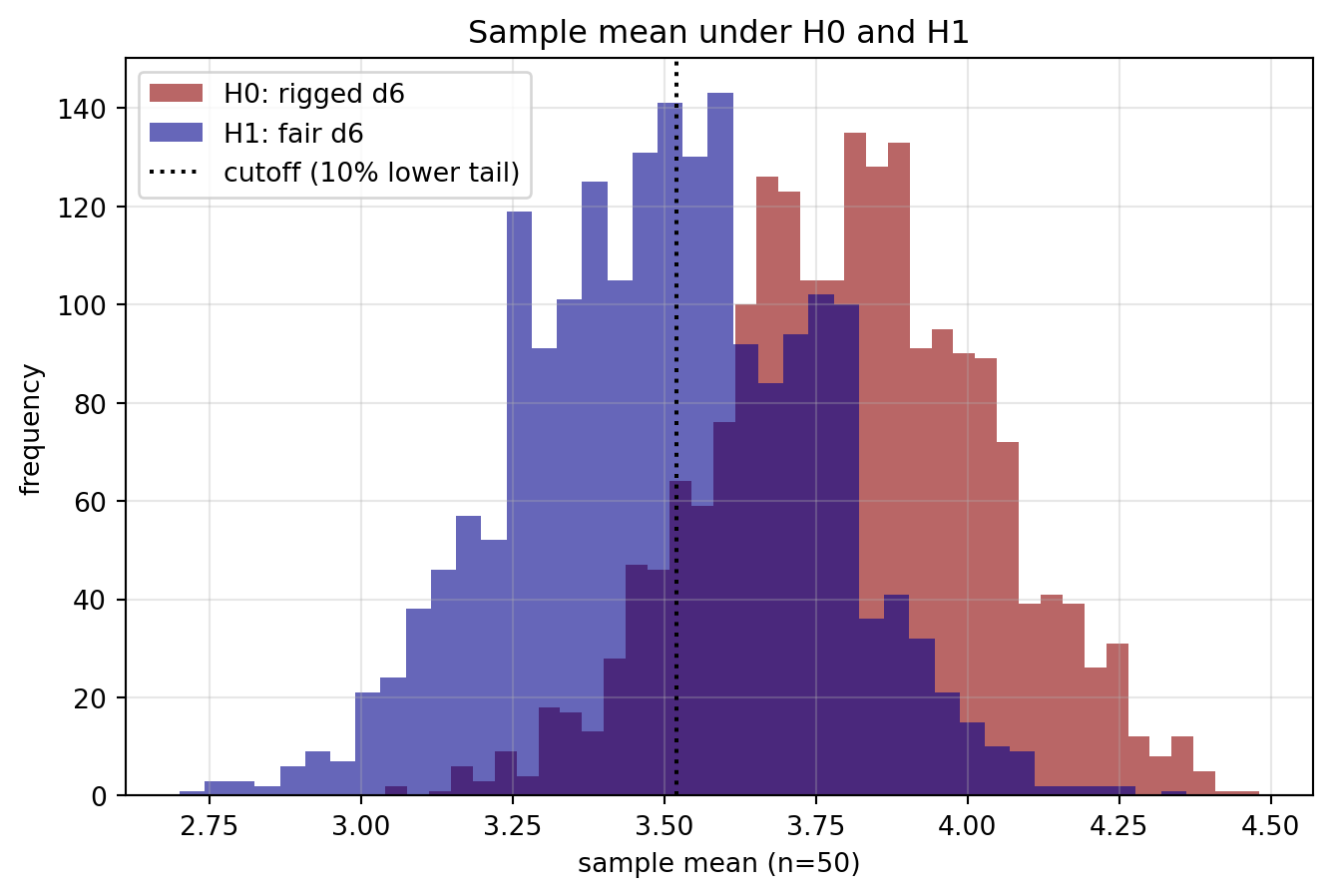
Trial 01 | fair   | test statistic=3.260000 | p-value=0.011 | reject H0          | correct
Trial 02 | fair   | test statistic=3.600000 | p-value=0.192 | fail to reject H0  | type II error
Trial 03 | fair   | test statistic=3.500000 | p-value=0.090 | reject H0          | correct
Trial 04 | rigged | test statistic=3.740000 | p-value=0.400 | fail to reject H0  | correct
Trial 05 | rigged | test statistic=3.600001 | p-value=0.195 | fail to reject H0  | correct
Trial 06 | fair   | test statistic=3.359999 | p-value=0.025 | reject H0          | correct
Trial 07 | fair   | test statistic=3.159999 | p-value=0.002 | reject H0          | correct
Trial 08 | fair   | test statistic=3.480001 | p-value=0.084 | reject H0          | correct
Trial 09 | fair   | test statistic=3.499999 | p-value=0.085 | reject H0          | correct
Trial 10 | rigged | test statistic=3.800000 | p-value=0.498 | fail to reject H0  | correct
Trial 11 | fair   | test statistic=3.660001 | p-value=0.271 | fail to reject H0  | type II error
Trial 12 | rigged | test statistic=4.080000 | p-value=0.881 | fail to reject H0  | correct
Trial 13 | rigged | test statistic=3.420001 | p-value=0.049 | reject H0          | type I error
Trial 14 | rigged | test statistic=3.619999 | p-value=0.201 | fail to reject H0  | correct
Trial 15 | fair   | test statistic=3.499999 | p-value=0.086 | reject H0          | correct
Trial 16 | rigged | test statistic=3.800000 | p-value=0.500 | fail to reject H0  | correct
Trial 17 | fair   | test statistic=3.300000 | p-value=0.015 | reject H0          | correct
Trial 18 | rigged | test statistic=4.080000 | p-value=0.883 | fail to reject H0  | correct
Trial 19 | fair   | test statistic=3.160000 | p-value=0.003 | reject H0          | correct
Trial 20 | rigged | test statistic=4.179999 | p-value=0.945 | fail to reject H0  | correct
Trial 21 | rigged | test statistic=3.980000 | p-value=0.774 | fail to reject H0  | correct
Trial 22 | fair   | test statistic=2.780000 | p-value=0.000 | reject H0          | correct
Trial 23 | rigged | test statistic=3.879999 | p-value=0.614 | fail to reject H0  | correct
Trial 24 | rigged | test statistic=3.879999 | p-value=0.615 | fail to reject H0  | correct
Trial 25 | fair   | test statistic=3.120000 | p-value=0.001 | reject H0          | correct
Trial 26 | rigged | test statistic=4.000000 | p-value=0.799 | fail to reject H0  | correct
Trial 27 | rigged | test statistic=3.680001 | p-value=0.307 | fail to reject H0  | correct
Trial 28 | rigged | test statistic=3.860000 | p-value=0.594 | fail to reject H0  | correct
Trial 29 | rigged | test statistic=3.760001 | p-value=0.437 | fail to reject H0  | correct
Trial 30 | rigged | test statistic=3.940000 | p-value=0.722 | fail to reject H0  | correct
Frequency of type I errors: 0.1000
Frequency of type II errors: 0.4890
Empirical power: 0.5110
Comments on the results: Frequency of type I errors: 0.1000 is not a coincidence, it’s a tautology. Since we used the list test_statistics_H0 to compute the 10th percentile cutoff and we then asked “what fraction of observations fall under the 10th percentile?” it’s no surprise we should find “exactly 10%”.
Frequency of type II errors: 0.5220 means that when H1 was true (fair d6) we failed to reject the null 52.2% of the time.
Empirical power: 0.4780 is just a reformulation of the same result: when H1 was true (fair d6) we correctly rejected the null 47.8% of the time.
ImportantA common mistake
A common mistake when simulating trials is to divide the number of type I errors by the total number of trials (which include trials with a rigged d6 and trials with a fair d6).
trials=[{'trial': 1, 'true_type': 'Fair', 'statistic': 3.2399991908223433, 'p_value': 0.5805, 'decision': 'Reject H0', 'error': 'Correct (reject H0, die is fair)'}, {'trial': 2, 'true_type': 'Fair', 'statistic': 3.620000503022172, 'p_value': 0.8235, 'decision': 'Fail to reject H0', 'error': 'Type II error (fail to reject H0, die is fair)'}, {'trial': 3, 'true_type': 'Fair', 'statistic': 3.6800002960031724, 'p_value': 0.7325, 'decision': 'Fail to reject H0', 'error': 'Type II error (fail to reject H0, die is fair)'}, {'trial': 4, 'true_type': 'Rigged', 'statistic': 3.8399998484142364, 'p_value': 0.455, 'decision': 'Fail to reject H0', 'error': 'Correct (fail to reject H0, die is rigged)'}, {'trial': 5, 'true_type': 'Fair', 'statistic': 3.2199998369577267, 'p_value': 0.5555, 'decision': 'Reject H0', 'error': 'Correct (reject H0, die is fair)'}, {'trial': 6, 'true_type': 'Rigged', 'statistic': 3.659999193254471, 'p_value': 0.778, 'decision': 'Fail to reject H0', 'error': 'Correct (fail to reject H0, die is rigged)'}, {'trial': 7, 'true_type': 'Rigged', 'statistic': 3.560000493244195, 'p_value': 0.909, 'decision': 'Fail to reject H0', 'error': 'Correct (fail to reject H0, die is rigged)'}, {'trial': 8, 'true_type': 'Fair', 'statistic': 3.3999993981476893, 'p_value': 0.855, 'decision': 'Reject H0', 'error': 'Correct (reject H0, die is fair)'}, {'trial': 9, 'true_type': 'Rigged', 'statistic': 3.8400002699516524, 'p_value': 0.4505, 'decision': 'Fail to reject H0', 'error': 'Correct (fail to reject H0, die is rigged)'}, {'trial': 10, 'true_type': 'Fair', 'statistic': 3.1799995830902743, 'p_value': 0.4805, 'decision': 'Reject H0', 'error': 'Correct (reject H0, die is fair)'}, {'trial': 11, 'true_type': 'Rigged', 'statistic': 3.939999470813085, 'p_value': 0.298, 'decision': 'Fail to reject H0', 'error': 'Correct (fail to reject H0, die is rigged)'}, {'trial': 12, 'true_type': 'Rigged', 'statistic': 3.8399998444615937, 'p_value': 0.4555, 'decision': 'Fail to reject H0', 'error': 'Correct (fail to reject H0, die is rigged)'}, {'trial': 13, 'true_type': 'Fair', 'statistic': 3.459999288477834, 'p_value': 0.943, 'decision': 'Fail to reject H0', 'error': 'Type II error (fail to reject H0, die is fair)'}, {'trial': 14, 'true_type': 'Fair', 'statistic': 3.4399995217934007, 'p_value': 0.909, 'decision': 'Fail to reject H0', 'error': 'Type II error (fail to reject H0, die is fair)'}, {'trial': 15, 'true_type': 'Fair', 'statistic': 2.8999995700580037, 'p_value': 0.1075, 'decision': 'Reject H0', 'error': 'Correct (reject H0, die is fair)'}, {'trial': 16, 'true_type': 'Fair', 'statistic': 3.520000645663566, 'p_value': 0.965, 'decision': 'Fail to reject H0', 'error': 'Type II error (fail to reject H0, die is fair)'}, {'trial': 17, 'true_type': 'Fair', 'statistic': 3.42000038896801, 'p_value': 0.8955, 'decision': 'Fail to reject H0', 'error': 'Type II error (fail to reject H0, die is fair)'}, {'trial': 18, 'true_type': 'Rigged', 'statistic': 3.939999007183462, 'p_value': 0.3035, 'decision': 'Fail to reject H0', 'error': 'Correct (fail to reject H0, die is rigged)'}, {'trial': 19, 'true_type': 'Fair', 'statistic': 3.5400000175298083, 'p_value': 0.952, 'decision': 'Fail to reject H0', 'error': 'Type II error (fail to reject H0, die is fair)'}, {'trial': 20, 'true_type': 'Rigged', 'statistic': 3.9400009181558393, 'p_value': 0.274, 'decision': 'Fail to reject H0', 'error': 'Correct (fail to reject H0, die is rigged)'}, {'trial': 21, 'true_type': 'Rigged', 'statistic': 3.9799990468692874, 'p_value': 0.235, 'decision': 'Fail to reject H0', 'error': 'Correct (fail to reject H0, die is rigged)'}, {'trial': 22, 'true_type': 'Rigged', 'statistic': 4.099999883870432, 'p_value': 0.112, 'decision': 'Fail to reject H0', 'error': 'Correct (fail to reject H0, die is rigged)'}, {'trial': 23, 'true_type': 'Fair', 'statistic': 3.9400004805157547, 'p_value': 0.2805, 'decision': 'Fail to reject H0', 'error': 'Type II error (fail to reject H0, die is fair)'}, {'trial': 24, 'true_type': 'Rigged', 'statistic': 3.9800005222108443, 'p_value': 0.218, 'decision': 'Fail to reject H0', 'error': 'Correct (fail to reject H0, die is rigged)'}, {'trial': 25, 'true_type': 'Fair', 'statistic': 3.580000750366518, 'p_value': 0.879, 'decision': 'Fail to reject H0', 'error': 'Type II error (fail to reject H0, die is fair)'}, {'trial': 26, 'true_type': 'Rigged', 'statistic': 3.579999518066288, 'p_value': 0.898, 'decision': 'Fail to reject H0', 'error': 'Correct (fail to reject H0, die is rigged)'}, {'trial': 27, 'true_type': 'Fair', 'statistic': 3.620000206672979, 'p_value': 0.827, 'decision': 'Fail to reject H0', 'error': 'Type II error (fail to reject H0, die is fair)'}, {'trial': 28, 'true_type': 'Rigged', 'statistic': 4.239999777077628, 'p_value': 0.0325, 'decision': 'Reject H0', 'error': 'Type I error (reject H0, die is rigged)'}, {'trial': 29, 'true_type': 'Fair', 'statistic': 3.1799998181483122, 'p_value': 0.484, 'decision': 'Reject H0', 'error': 'Correct (reject H0, die is fair)'}, {'trial': 30, 'true_type': 'Rigged', 'statistic': 3.8599996894897597, 'p_value': 0.4195, 'decision': 'Fail to reject H0', 'error': 'Correct (fail to reject H0, die is rigged)'}]

# Compute error frequencies and empirical power
print("\n" + "="*50)
print("ERROR FREQUENCY ANALYSIS")
print("="*50)

# Count error types from the trials
typeI_count = sum(1 for t in trials if t['error'] == 'Type I error (reject H0, die is rigged)')
typeII_count = sum(1 for t in trials if t['error'] == 'Type II error (fail to reject H0, die is fair)')
correct_count = 30 - typeI_count - typeII_count

# Calculate frequencies
typeI_freq = typeI_count / 30  ### LB: this is incorrect
typeII_freq = typeII_count / 30  ### LB: this is incorrect
empirical_power = 1 - typeII_freq

print(f"Total trials: 30")
print(f"Correct decisions: {correct_count} ({correct_count/30:.2%})")
print(f"Type I errors: {typeI_count} ({typeI_freq:.2%})")
print(f"Type II errors: {typeII_count} ({typeII_freq:.2%})")
print(f"\nEmpirical power of the test: {empirical_power:.2%}")

print(f"\nExpected Type I error rate (alpha): {alpha:.2%}")
print(f"Observed Type I error rate: {typeI_freq:.2%}")
==================================================
ERROR FREQUENCY ANALYSIS
==================================================
Total trials: 30
Correct decisions: 19 (63.33%)
Type I errors: 1 (3.33%)
Type II errors: 10 (33.33%)

Empirical power of the test: 66.67%

Expected Type I error rate (alpha): 10.00%
Observed Type I error rate: 3.33%
The frequency of type I errors is the empirical counterpart of a conditional probability, conditional on H0 being true. The frequency of type II errors is the empirical counterpart of a conditional probability, conditional on H0 being false. So the denominators should not be the total number of trials (which include trials with a rigged d6 and trials with a fair d6).
Instead:
frequency of type I errors is the number of type I errors divided by the number of rigged d6 (H0 is true) trials.
frequency of type II errors is the number of type II errors divided by the number of fair d6 (H0 is false) trials.
16610101020 Hypothesis testing — Mean vs Variance (OPTIONAL: vs log likelihood ratio)
The goal of this exercise is to consider a different type of rigged d6 and different test statistics. The null hypothesis is H0: the d6 is fair, and the alternative hypothesis is H1: the d6 is rigged.
Start your code with:
import random
random.seed(16610101020)

n_simulations = 3000
alpha = 0.10
sample_size = 50

interval_widths_fair = [12, 12, 12, 12, 12, 12]
interval_widths_rigged = [16, 6, 10, 10, 10, 20]

def jitter(x, scale):
    return x + random.uniform(-scale, scale)
Apply a small jitter (1e-6) whenever you compute a test statistic. The jitter ensures that no two samples have exactly the same value of the test statistic.
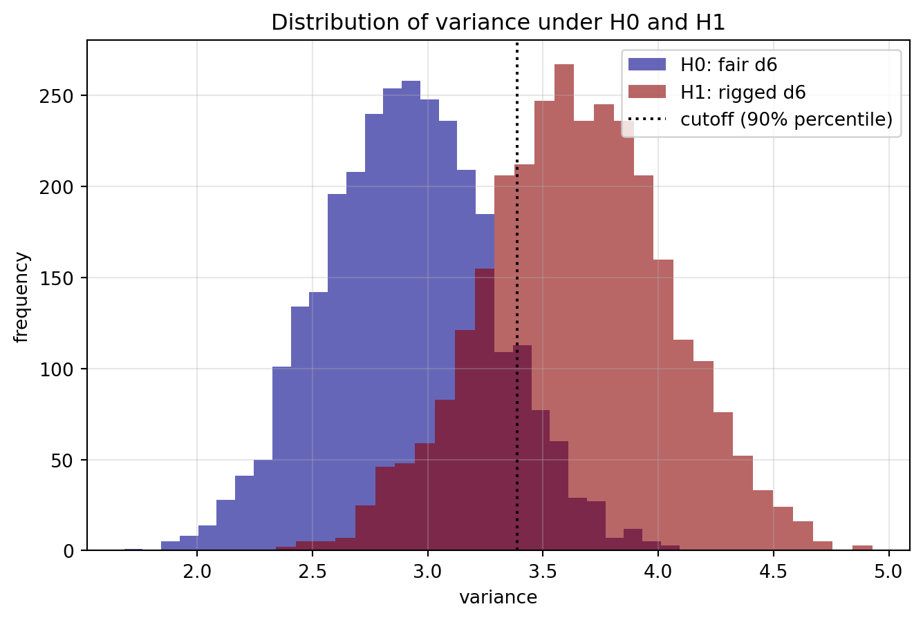
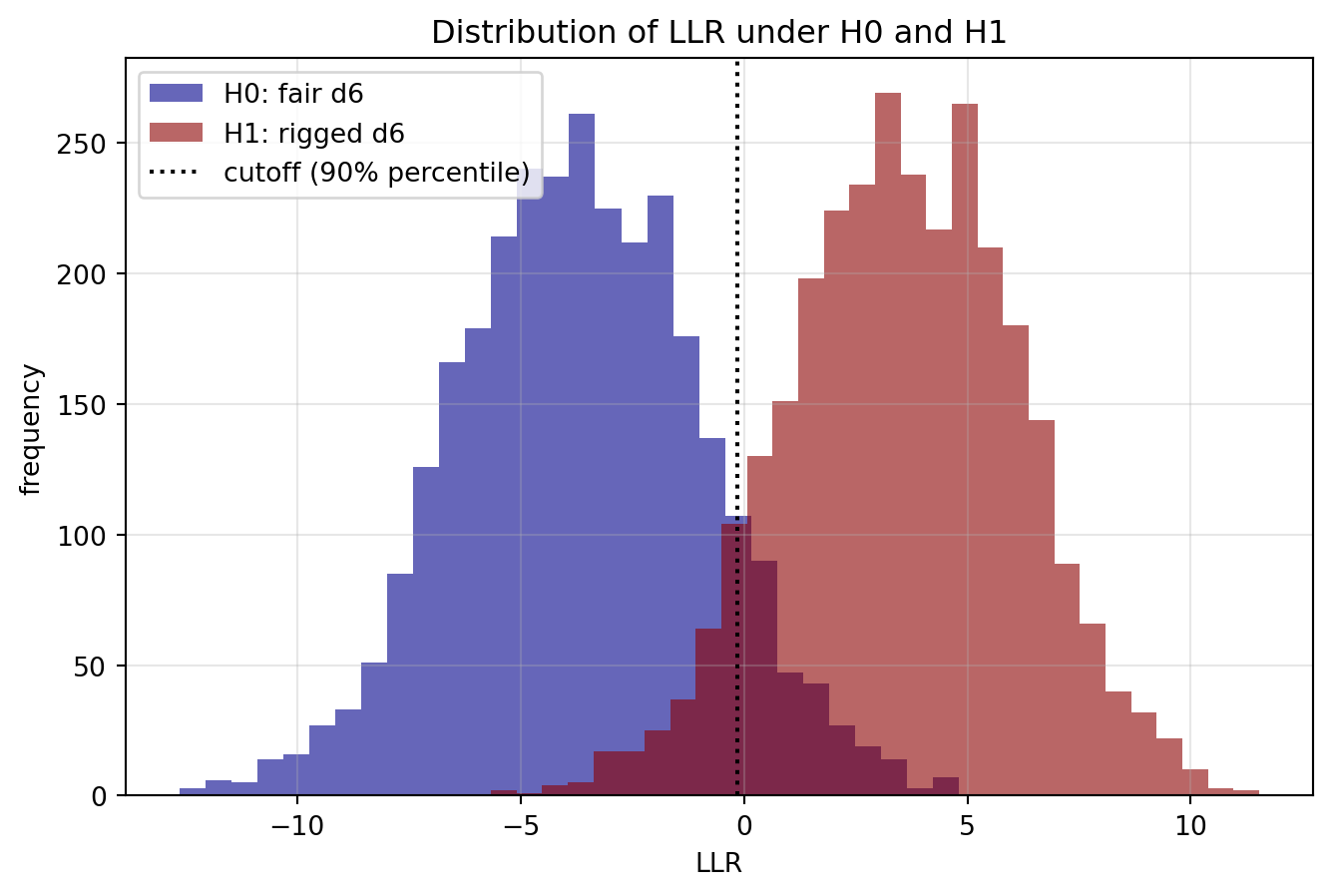
Follow the hypothesis testing procedure outlined below, using the sample mean as the test statistic (as in the lecture notes). Then, repeat the procedure, with a different test statistic: the sample variance. OPTIONAL: repeat the procedure with yet another test statistic: the log-likelihood ratio.
Remark: you can compute multiple test statistics on the same sample, rather than draw new samples when you change the test statistic. At the end, construct a dataframe with one row per test statistic, and with columns for:
decision rule (cutoff)
frequency of type I errors (empirical alpha)
frequency of type II errors
empirical power of the test statistic
Sort the dataframe by decreasing empirical power and print the dataframe.
TipHypothesis testing procedure
Distribution of the test statistic and decision rule.
Draw
n_simulationssamples assuming H0 and compute the test statistic for each sample.Display the distribution of the test statistic under H0 as a histogram.
Draw
n_simulationssamples assuming H1 and compute the test statistic for each sample.Display the distribution of the test statistic under H1 as a histogram on the same graph.
Choose the decision rule (the rejection region) such that when H0 is true, type I errors occur with probability
alpha.
From trials to simulations
Using the fair d6 samples drawn previously, compute the frequency of type I errors.
Using the rigged d6 samples drawn previously, compute the frequency of type II errors.
Give the empirical power of the test.
import random
random.seed(16610101020)

n_simulations = 3000
alpha = 0.10
sample_size = 50

interval_widths_fair = [12, 12, 12, 12, 12, 12]
interval_widths_rigged = [16, 6, 10, 10, 10, 20]

def jitter(x, scale):
    return x + random.uniform(-scale, scale)


import math
import matplotlib.pyplot as plt
import pandas as pd


#%% Construct the fair and rigged d6

assert sum(interval_widths_fair) == 72
assert sum(interval_widths_rigged) == 72


thresholds_fair = []
running_total = 0

for interval_width in interval_widths_fair:
    running_total += interval_width
    thresholds_fair.append(running_total)


thresholds_rigged = []
running_total = 0

for interval_width in interval_widths_rigged:
    running_total += interval_width
    thresholds_rigged.append(running_total)


probabilities_fair = []

for interval_width in interval_widths_fair:
    probabilities_fair.append(interval_width / 72)


probabilities_rigged = []

for interval_width in interval_widths_rigged:
    probabilities_rigged.append(interval_width / 72)


def roll_fair_d6():

    draw = random.randint(1, 72)

    for face, threshold in enumerate(thresholds_fair, start=1):
        if draw <= threshold:
            return face


def roll_rigged_d6():

    draw = random.randint(1, 72)

    for face, threshold in enumerate(thresholds_rigged, start=1):
        if draw <= threshold:
            return face


#%% Define the test statistics
### Computing sample_mean and sample_variance by hand is not necessary,
### you could simply use a command for them
## statistics.mean, np.mean are commands which can be applied to lists
## alternatively, numpy arrays are endowed with a method .mean()
## pandas data series are also endowed with a method .mean()

def sample_mean(sample):

    mean = sum(sample) / len(sample)

    return jitter(mean, 1e-6)


def sample_variance(sample):

    mean = sum(sample) / len(sample)

    squared_deviations = []

    for observation in sample:
        squared_deviation = (observation - mean) ** 2
        squared_deviations.append(squared_deviation)

    variance = sum(squared_deviations) / (len(sample) - 1)

    return jitter(variance, 1e-6)


def log_likelihood_ratio(sample):

    total = 0

    for observation in sample:
        probability_H1 = probabilities_rigged[observation - 1]
        probability_H0 = probabilities_fair[observation - 1]

        total += math.log(probability_H1 / probability_H0)

    return jitter(total, 1e-6)


#%% Generate samples under H0 and H1

# H0: the d6 is fair
# H1: the d6 is rigged

samples_H0 = []
samples_H1 = []

for i_simulation in range(n_simulations):

    sample_H0 = []

    for i_roll in range(sample_size):
        sample_H0.append(roll_fair_d6())

    samples_H0.append(sample_H0)


    sample_H1 = []

    for i_roll in range(sample_size):
        sample_H1.append(roll_rigged_d6())

    samples_H1.append(sample_H1)


#%% Compute all test statistics using the same samples

statistics = {
    "mean": {
        "H0": [],
        "H1": []
    },
    "variance": {
        "H0": [],
        "H1": []
    },
    "LLR": {
        "H0": [],
        "H1": []
    }
}


for sample in samples_H0:

    statistics["mean"]["H0"].append(
        sample_mean(sample)
    )

    statistics["variance"]["H0"].append(
        sample_variance(sample)
    )

    statistics["LLR"]["H0"].append(
        log_likelihood_ratio(sample)
    )


for sample in samples_H1:

    statistics["mean"]["H1"].append(
        sample_mean(sample)
    )

    statistics["variance"]["H1"].append(
        sample_variance(sample)
    )

    statistics["LLR"]["H1"].append(
        log_likelihood_ratio(sample)
    )


#%% Distributions, decision rules, errors and power

rows = []
cutoffs = {}

for statistic_name, distributions in statistics.items():

    statistics_H0 = distributions["H0"]
    statistics_H1 = distributions["H1"]

    cutoff_index = int((1 - alpha) * n_simulations)
    cutoff = sorted(statistics_H0)[cutoff_index]

    cutoffs[statistic_name] = cutoff

    # Display the distributions under H0 and H1 on the same graph

    plt.figure(figsize=(8, 5))

    plt.hist(
        statistics_H0,
        bins=30,
        alpha=0.6,
        color="darkblue",
        label="H0: fair d6"
    )

    plt.hist(
        statistics_H1,
        bins=30,
        alpha=0.6,
        color="darkred",
        label="H1: rigged d6"
    )

    plt.axvline(
        cutoff,
        color="black",
        linestyle=":",
        label=f"cutoff ({1 - alpha:.0%} percentile)"
    )

    plt.xlabel(statistic_name)
    plt.ylabel("frequency")
    plt.title(f"Distribution of {statistic_name} under H0 and H1")
    plt.legend()
    plt.grid(alpha=0.3)

    plt.show()


    # Type I error:
    # reject H0 when the d6 is fair

    number_type_I_errors = 0

    for test_statistic in statistics_H0:
        if test_statistic >= cutoff:
            number_type_I_errors += 1

    frequency_type_I_errors = (
        number_type_I_errors / n_simulations
    )


    # Type II error:
    # fail to reject H0 when the d6 is rigged

    number_type_II_errors = 0

    for test_statistic in statistics_H1:
        if test_statistic < cutoff:
            number_type_II_errors += 1

    frequency_type_II_errors = (
        number_type_II_errors / n_simulations
    )


    # Power:
    # reject H0 when the d6 is rigged

    empirical_power = 1 - frequency_type_II_errors


    rows.append({
        "test_statistic": statistic_name,
        "cutoff": f"{cutoff:.4f}",
        "freq_type_I": frequency_type_I_errors,
        "freq_type_II": frequency_type_II_errors,
        "empirical_power": empirical_power
    })


#%% Construct and sort the results dataframe

results_df = pd.DataFrame(rows)

results_df = results_df.sort_values(
    by="empirical_power",
    ascending=False
)

results_df = results_df.reset_index(drop=True)

print(results_df)

### Comment
# =============================================================================
# #   test_statistic   cutoff  freq_type_I  freq_type_II  empirical_power
# # 0            LLR  -0.1441          0.1      0.075333         0.924667
# # 1       variance   3.3894          0.1      0.264333         0.735667
# # 2           mean   3.8200          0.1      0.631000         0.369000
# =============================================================================

## all test statistics have the same alpha = 0.1,
## so the comparison is fair, and it shows that the
## LLR test achieves the highest empirical_power 0.92,
## followed by the variance test with 0.74
## the means test is last with 0.37.

## this quantifies the graphical intuition: the amount of separation
## (lack of overlap) in the histograms of test statistics under H0 and H1
## is directly related to the empirical power of the test statistics.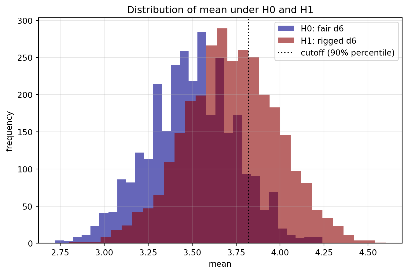
  test_statistic   cutoff  freq_type_I  freq_type_II  empirical_power
0            LLR  -0.1441          0.1      0.075333         0.924667
1       variance   3.3894          0.1      0.264333         0.735667
2           mean   3.8200          0.1      0.631000         0.369000
Exercise 1200110030 — Pooled virus testing
Source: Cyganowski, S., Kloeden, P. E., and Ombach, J. (2002), From Elementary Probability to Stochastic Differential Equations with Maple, Springer.
Start your code with:
import random
random.seed(1200110030)

n_simulations = 1400
p_infected = 0.01
n_population=1200
A population of n_population individuals is screened for a rare virus. The probability that a given individual is infected is p_infected, independent across individuals. The testing procedure is excellent (no false positives or false negatives), but expensive, so in an effort to reduce costs, the testing center practices pooled testing:
divide the population into groups of 30 individuals (pools).
take half the blood sample (5mL out of 10mL) of every individual within a group and mix them together.
test the mixed blood
if the mixed blood test is negative, the group is “clean”.
if the mixed blood test is positive, test separately and individually the remaining 5mL of blood from every individual in the group.
One simulation of one testing campaign.
Simulate one testing campaign: generate a sample with n_population individuals, each with a status (is_infected=True or is_infected=False) generated randomly using probability p_infected, and assume that individuals 0 through 29 form one group, then individuals 30 through 59 another group, etc.
Print:
the number of clean groups (tests performed of mixed blood which were negative)
the number of groups with at least one infected individual (tests performed of mixed blood which were positive)
the total number of group tests performed
the total number of individual tests performed
the total number of tests performed
Multiple simulations
Simulate a testing campaign n_simulations times: in each simulation, generate a new sample, then conduct the testing campaign. For each simulation, store the total number of tests performed.
Print descriptive statistics on the total number of tests:
average
minimum
25th percentile
median
75th percentile
maximum
Choosing the group size optimally
We are interested in whether dividing the population into groups of 30 is optimal, or whether a different number would reduce the expected cost of testing the entire population. We want to simulate testing campaigns assuming different group sizes: 2, 6, 8, 10, 12, 14, 16, 20, 25, 32, 40, 48.
For each possible group size, simulate the testing campaign n_simulations times.
Construct a dataframe where each row is a group size, and different columns display:
the minimum number of tests across simulations
the average number of tests across simulations
the maximum number of tests across simulations
Print the group size with the lowest average number of tests.
OPTIONAL: run the code again with a lower probability of infection p_infected = 0.005. How does the optimal group size change?
# -*- coding: utf-8 -*-
"""
Created on Tue Sep  8 20:31:18 2026

@author: lb222
"""

import random
random.seed(1200110030)

n_simulations = 1400
p_infected = 0.01
n_population=1200


import matplotlib.pyplot as plt
import pandas as pd


#%% Function for one pooled-testing campaign

def testing_campaign(population, group_size):

    number_clean_groups = 0
    number_positive_groups = 0
    number_group_tests = 0
    number_individual_tests = 0

    # Individuals are placed into consecutive groups.
    # The final group contains whoever is left.

    for group_start in range(0, len(population), group_size):

        group_end = group_start + group_size
        group = population[group_start:group_end]

        # One mixed-blood test is performed for each group.

        number_group_tests += 1

        if True in group:

            number_positive_groups += 1

            # If the group test is positive, every individual
            # in that group is tested separately.

            number_individual_tests += len(group)

        else:

            number_clean_groups += 1

    total_number_tests = (
        number_group_tests
        + number_individual_tests
    )

    results = {
        "number_clean_groups": number_clean_groups,
        "number_positive_groups": number_positive_groups,
        "number_group_tests": number_group_tests,
        "number_individual_tests": number_individual_tests,
        "total_number_tests": total_number_tests
    }

    return results


#%% One simulation of one testing campaign

population = []

for individual in range(n_population):

    is_infected = random.random() < p_infected
    population.append(is_infected)


results = testing_campaign(
    population=population,
    group_size=30
)


print(
    "Number of clean groups:",
    results["number_clean_groups"]
)

print(
    "Number of groups with at least one infected individual:",
    results["number_positive_groups"]
)

print(
    "Total number of mixed blood tests performed:",
    results["number_group_tests"]
)

print(
    "Total number of individual blood tests performed:",
    results["number_individual_tests"]
)

print(
    "Total number of tests performed:",
    results["total_number_tests"]
)


#%% Multiple simulations

total_tests_all_simulations = []

for i_simulation in range(n_simulations):

    population = []

    for individual in range(n_population):

        is_infected = random.random() < p_infected
        population.append(is_infected)

    results = testing_campaign(
        population=population,
        group_size=30
    )

    total_tests_all_simulations.append(
        results["total_number_tests"]
    )


total_tests_series = pd.Series(
    total_tests_all_simulations,
    name="total_number_tests"
)

descriptive_statistics = total_tests_series.describe()

print()
print("Descriptive statistics for the total number of tests:")

print(
    descriptive_statistics.to_string(
        float_format="%.4f"
    )
)


#%% Choosing the group size optimally

group_sizes = [
    2, 3, 4, 5, 6, 7, 8, 9, 10, 11, 12, 13, 14,
    15, 16, 17, 18, 19, 20, 21, 22, 25, 32, 40, 48
]

rows = []

for group_size in group_sizes:

    total_tests_group_size = []
    mixed_tests_group_size = []
    positive_mixed_tests_group_size = []
    individual_tests_group_size = []

    for i_simulation in range(n_simulations):

        population = []

        for individual in range(n_population):

            is_infected = random.random() < p_infected
            population.append(is_infected)

        results = testing_campaign(
            population=population,
            group_size=group_size
        )

        total_tests_group_size.append(
            results["total_number_tests"]
        )

        mixed_tests_group_size.append(
            results["number_group_tests"]
        )

        positive_mixed_tests_group_size.append(
            results["number_positive_groups"]
        )

        individual_tests_group_size.append(
            results["number_individual_tests"]
        )

    total_tests_series = pd.Series(
        total_tests_group_size
    )

    mixed_tests_series = pd.Series(
        mixed_tests_group_size
    )

    positive_mixed_tests_series = pd.Series(
        positive_mixed_tests_group_size
    )

    individual_tests_series = pd.Series(
        individual_tests_group_size
    )

    proportion_positive_mixed_tests = (
        positive_mixed_tests_series.sum()
        / mixed_tests_series.sum()
    )

    rows.append({
        "group_size": group_size,
        "proportion_positive_mixed_tests": proportion_positive_mixed_tests,
        "average_mixed_tests": mixed_tests_series.mean(),
        "average_individual_tests": individual_tests_series.mean(),
        "average_total_tests": total_tests_series.mean(),
        "minimum_total_tests": total_tests_series.min(),
        "maximum_total_tests": total_tests_series.max()
    })


results_df = pd.DataFrame(rows)


print()
print("Results by group size:")

display_labels = [
    "size",
    "pos_mx_freq",
    "avg_mx",
    "avg_ind",
    "avg_tot",
    "min_tot",
    "max_tot"
]

print(
    results_df.to_string(
        index=False,
        header=display_labels,
        formatters={
            "proportion_positive_mixed_tests": "{:.4f}".format,
            "average_mixed_tests": "{:.2f}".format,
            "average_individual_tests": "{:.2f}".format,
            "average_total_tests": "{:.2f}".format
        }
    )
)
#%% Find the group size with the lowest average number of tests

optimal_row = results_df.loc[
    results_df["average_total_tests"].idxmin()
]

optimal_group_size = int(
    optimal_row["group_size"]
)

lowest_average_tests = optimal_row["average_total_tests"]


print()

print(
    f"The group size with the lowest average number of tests "
    f"is {optimal_group_size}."
)

print(
    f"Its average number of tests is "
    f"{lowest_average_tests:.4f}."
)


#%% Plot the two components of the average number of tests

plt.figure(figsize=(9, 6))

plt.scatter(
    results_df["group_size"],
    results_df["average_mixed_tests"],
    color="darkblue",
    label="Average mixed blood tests"
)

plt.plot(
    results_df["group_size"],
    results_df["average_mixed_tests"],
    color="darkblue",
    alpha=0.5
)

plt.scatter(
    results_df["group_size"],
    results_df["average_individual_tests"],
    color="darkred",
    label="Average individual blood tests"
)

plt.plot(
    results_df["group_size"],
    results_df["average_individual_tests"],
    color="darkred",
    alpha=0.5
)

plt.scatter(
    results_df["group_size"],
    results_df["average_total_tests"],
    color="black",
    label="Average total tests"
)

plt.plot(
    results_df["group_size"],
    results_df["average_total_tests"],
    color="black",
    alpha=0.5
)

plt.xlabel("Group size")
plt.ylabel("Average number of tests")

plt.title(
    f"Mixed, individual, and total tests across "
    f"{n_simulations} simulations"
)

plt.grid(alpha=0.3)
plt.legend()

plt.show()


#%% OPTIONAL: repeat with a lower infection probability

# Change the parameter near the beginning of the code to:
#
# p_infected = 0.005
#
# Then run the code again and compare the group size with
# the lowest average number of tests.
Number of clean groups: 31
Number of groups with at least one infected individual: 9
Total number of mixed blood tests performed: 40
Total number of individual blood tests performed: 270
Total number of tests performed: 310
Descriptive statistics for the total number of tests:
count 1400.0000
mean 347.5857
std 82.2366
min 100.0000
25% 280.0000
50% 340.0000
75% 400.0000
max 610.0000
Results by group size:
size pos_mx_freq avg_mx avg_ind avg_tot min_tot max_tot
2 0.0199 600.00 23.88 623.88 606 650
3 0.0296 400.00 35.53 435.53 406 481
4 0.0389 300.00 46.64 346.64 312 396
5 0.0487 240.00 58.48 298.48 255 370
6 0.0583 200.00 69.96 269.96 218 356
7 0.0678 172.00 81.56 253.56 193 361
8 0.0773 150.00 92.75 242.75 174 326
9 0.0867 134.00 104.42 238.42 161 377
10 0.0954 120.00 114.49 234.49 150 340
11 0.1038 110.00 125.50 235.50 143 374
12 0.1152 100.00 138.26 238.26 124 376
13 0.1208 93.00 145.76 238.76 119 405
14 0.1326 86.00 159.24 245.24 128 422
15 0.1405 80.00 168.55 248.55 110 425
16 0.1482 75.00 177.90 252.90 107 443
17 0.1566 71.00 188.35 259.35 122 445
18 0.1647 67.00 197.86 264.86 121 463
19 0.1724 64.00 209.06 273.06 102 482
20 0.1819 60.00 218.29 278.29 120 440
21 0.1888 58.00 229.40 287.40 100 478
22 0.1961 55.00 236.22 291.22 99 517
25 0.2251 48.00 270.09 318.09 123 573
32 0.2717 38.00 327.83 365.83 102 646
40 0.3323 30.00 398.80 428.80 110 830
48 0.3824 25.00 458.85 483.85 121 841
The group size with the lowest average number of tests is 10.
Its average number of tests is 234.4929.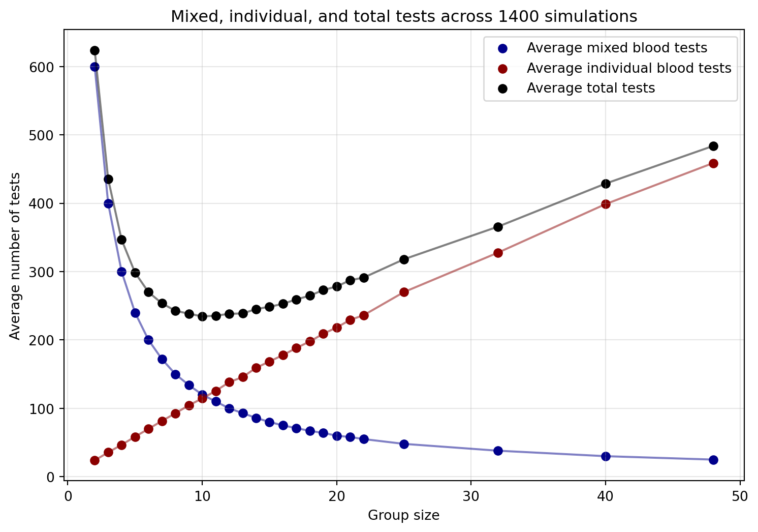
The plot illustrates the tradeoff governing group size:
A small group size increases the probability that any given mixed blood test is negative, and even when the test is positive, the number of follow-up individual tests will be small, but a small group size implies testing many mixed blood samples.
A large group size makes it more likely that any given mixed blood test is positive, requiring many follow-up individual tests.
A group size around 10 achieves a good balance, and leads to the lowest average number of tests.