Univariate Statistics

Coding, simulations, lists, samples, descriptive statistics, hypothesis testing, power

Setup: imports and random number generator seed

In The Effect

simulated data https://theeffectbook.net/ch-Identification.html#the-data-generating-process
data generating process https://theeffectbook.net/ch-Identification.html#the-data-generating-process

First, we need python to import the random library so we have access to random number generators. We will also set an explicit seed for the random number generator. Setting a seed guarantees that the generator returns the same numbers each time it is invoked, so our results stay the same each time we execute this script, as long as we do so in the same set sequence.

import random
random.seed(12345)

Let us start with a simple virtual coin toss.

Coin toss: first attempt.

coin_1 = random.randint(0, 1)
print(coin_1)

Coin toss: another one!

coin_2 = random.randint(0, 1)
print(coin_2)

Our simple coin toss uses the function randint from the python library random. If we open the documentation, we find that randint(a, b) returns a random integer between a and b, including both endpoints. In our case, we use randint(0, 1), which means the function returns either 0 or 1 with equal probability. This gives us a simple way to represent the two possible outcomes of a fair coin toss.

Returning a more familiar “Heads or Tails”

coin = random.randint(0, 1)
if coin == 0:
    coin_face = "Heads"
else:
    coin_face = "Tails"
print(coin_face)

Tails

Best-of-five anyone?

For a best-of-five, we will hold the printing until the end, by appending each result to a string. Strings are collections of characters (for example, words or sentences enclosed in quotes such as “Heads” or “Tails” or “This is a string”). You can concatenate strings by using the operator +. For example: “Heads” + “,” + “Tails” produces the string “Heads, Tails”. We will also use the operator +=, which means “take the current value of the variable and add something to it”. In other words, x += y is a shorter way of writing x = x + y. Each time we update our string with +=, we are extending it by adding new content at the end.

We will also use a for loop, which is a way to instruct python to repeat the same block of code several times in sequence.

coin_face_sequence = "" # initialize an empty string

for coin_toss in range(5):
    coin = random.randint(0, 1)
    if coin == 0:
        coin_face_sequence += "Heads, "
    else:
        coin_face_sequence += "Tails, "

print(coin_face_sequence)

Tails, Heads, Tails, Tails, Heads,

Another best-of-five

coin_face_sequence = ""

for coin_toss in range(5):
    coin = random.randint(0, 1)
    if coin == 0:
        coin_face_sequence += "Heads, "
    else:
        coin_face_sequence += "Tails, "

print(coin_face_sequence)

Tails, Heads, Tails, Tails, Heads,

Wait, that is just the same sequence again!

Another, just to be sure

coin_face_sequence = ""

for coin_toss in range(5):
    coin = random.randint(0, 1)
    if coin == 0:
        coin_face_sequence += "Heads, "
    else:
        coin_face_sequence += "Tails, "

print(coin_face_sequence)

Heads, Tails, Heads, Tails, Heads,

OK, so at least we know it is not always giving us the same sequence.

Off-ramp: random number generator seed

Let us experiment a bit with the seed, to understand better what it does.

random.seed(123)
print("\n random.seed has just been reset")

coin_face_sequence = ""

for coin_toss in range(8):
    coin = random.randint(0, 1)
    if coin == 0:
        coin_face_sequence += "Heads, "
    else:
        coin_face_sequence += "Tails, "

print(coin_face_sequence)


 random.seed has just been reset
Heads, Tails, Heads, Tails, Tails, Heads, Heads, Tails,

random.seed(123)
print("\n random.seed has just been reset AGAIN")

coin_face_sequence = ""

for coin_toss in range(8):
    coin = random.randint(0, 1)
    if coin == 0:
        coin_face_sequence += "Heads, "
    else:
        coin_face_sequence += "Tails, "

print(coin_face_sequence)


 random.seed has just been reset AGAIN
Heads, Tails, Heads, Tails, Tails, Heads, Heads, Tails,

print("\n random.seed has NOT been reset")

coin_face_sequence = ""

for coin_toss in range(8):
    coin = random.randint(0, 1)
    if coin == 0:
        coin_face_sequence += "Heads, "
    else:
        coin_face_sequence += "Tails, "

print(coin_face_sequence)


 random.seed has NOT been reset
Tails, Tails, Heads, Heads, Heads, Tails, Tails, Heads,

The random number generator is deterministic. Once we fix the seed at the beginning of a script, the same sequence of values will then always be the same, as long as we follow the same sequence of calls.

Setting a seed ensures reproducibility of simulation methods.

That was probably enough coin tosses for one day. We need to roll dice.

Rolling a d6

In The Effect

variable https://theeffectbook.net/ch-DescribingVariables.html#descriptions-of-variables
observation https://theeffectbook.net/ch-DescribingVariables.html#summarizing-the-distribution
distribution https://theeffectbook.net/ch-DescribingVariables.html#the-distribution
theoretical distribution https://theeffectbook.net/ch-DescribingVariables.html#theoretical-distributions
categorical https://theeffectbook.net/ch-DescribingVariables.html#types-of-variables

randint(1, 6) returns one of the values 1, 2, 3, 4, 5, or 6, each with equal probability, simulating a fair six-sided die (also known as a d6).

roll_d6 = random.randint(1, 6)
print(roll_d6)

Repeated d6 rolls (manual observation)

Before moving to repeated rolling, a point of python convention: we always start counting at 0, not at 1. It can be confusing to mix code conventions and plain English, e.g. “first” being associated with index 0. We can use the inelegant but hopefully clearer 0-th, 1-th, 2-th in text to indicate python indexing. For example,

roll_the_string= "roll"  # a string
print("The 0-th character in the string is:   ", roll_the_string[0])
roll_the_list= ["r", "o", "l", "l"] ## a list of strings
print("The 1-th element in", roll_the_list, "is", roll_the_list[1])
d6_faces= [1, 2, 3, 4, 5, 6] ## a list of integers
print("The 2-th element in", d6_faces, "is", d6_faces[2])

The 0-th character in the string is:    r
The 1-th element in ['r', 'o', 'l', 'l'] is o
The 2-th element in [1, 2, 3, 4, 5, 6] is 3

Rolling a d6, 4 times

roll_0 = random.randint(1, 6)
roll_1 = random.randint(1, 6)
roll_2 = random.randint(1, 6)
roll_3 = random.randint(1, 6)

print(roll_0, roll_1, roll_2, roll_3)

1 4 1 5

This code works, but it is repetitive. We will improve this shortly.

Create empty list

results = []
print(results)

[]

Append to a list

roll_0 = random.randint(1, 6)
results.append(roll_0)
print(results)

[4]

roll_1 = random.randint(1, 6)
results.append(roll_1)
print(results)

[4, 1]

roll_2 = random.randint(1, 6)
results.append(roll_2)
print(results)

[4, 1, 1]

roll_3 = random.randint(1, 6)
results.append(roll_3)
print(results)

[4, 1, 1, 3]

Inspect sample size (length of a list)

length_results = len(results)
print("We have completed", length_results, "rolls.")

We have completed 4 rolls.

Inspect values

print("The 0-th roll resulted in a", results[0], ".")
print("The 1-th roll resulted in a", results[1], ".")

The 0-th roll resulted in a 4 .
The 1-th roll resulted in a 1 .

Off-ramp: variable semantics

What happens if we try to modify the 2-th roll?

roll_2 = random.randint(1, 6)
print(roll_2)
results.append(roll_2)
print(results)

6
[4, 1, 1, 3, 6]

Let’s try again, to understand why that did not work.

roll_2 = random.randint(1, 6)
print(roll_2)
results.append(roll_2)
print(results)

4
[4, 1, 1, 3, 6, 4]

If we were hoping to replace the 2-th (third in natural English counting) roll in the sequence, this did not work. There are two issues:

roll_2 makes sense to a human (or an LLM) as referring to the 2-th (third in natural English counting) roll in a sequence, but the machine only does what we ask. A name such as roll_2 is only a label chosen by the programmer. It suggests an order, but this order is not enforced by the structure of the program, we could equally well call the variable bob or roll55.
we used the .append method, which adds an element at the end of a list.

Lists can also be modified element by element. Here is another way to roll 4 times

roll_results = ["?", "?", "?", "?"]
print(roll_results)

roll = random.randint(1, 6)
roll_results[0] = roll
print(roll_results)

roll = random.randint(1, 6)
roll_results[1] = roll
print(roll_results)

## I did not enjoy this 1-th roll. It does not count. Try again.

roll = random.randint(1, 6)
roll_results[1] = roll
print(roll_results)

## This 1-th roll does not count either. Try again.

roll = random.randint(1, 6)
roll_results[1] = roll
print(roll_results)

## Much better.

roll = random.randint(1, 6)
roll_results[2] = roll
print(roll_results)

roll = random.randint(1, 6)
roll_results[3] = roll
print(roll_results)

['?', '?', '?', '?']
[1, '?', '?', '?']
[1, 1, '?', '?']
[1, 1, '?', '?']
[1, 6, '?', '?']
[1, 6, 2, '?']
[1, 6, 2, 2]

This approach allows us to: - assign values to specific positions, - modify values after they have been assigned, - treat the list as a fixed structure.

This also shows the difference between a cosmetic index such as roll_2 and a structural index such as roll_results[2]. roll_results[2] refers to the 2-th element inside the list roll_results: it always refers to the same location, and changing it modifies the list object itself.

Define function

At some point, we should try to automate all these d6 rolls. Writing functions allows us to reuse the same block of code with different inputs, instead of copying it multiple times.

def n_rolls_d6(n):
    results = []
    for i in range(n):
        roll = random.randint(1, 6)
        results.append(roll)
    return results

Generate a small sample

results_small = n_rolls_d6(4)
print(results_small)

[1, 3, 4, 5]

Inspect length of small sample

length_small = len(results_small)
print(length_small)

Generate a larger sample

results_large = n_rolls_d6(20)
print(results_large)

[4, 3, 4, 1, 3, 3, 5, 4, 2, 5, 6, 5, 5, 3, 1, 4, 6, 5, 4, 6]

Inspect length of large sample

length_large = len(results_large)
print(length_large)

Sort results

sorted_results = sorted(results_large)
print(sorted_results)

[1, 1, 2, 3, 3, 3, 3, 4, 4, 4, 4, 4, 5, 5, 5, 5, 5, 6, 6, 6]

Count ones

count_1 = sorted_results.count(1)
print(count_1)

Compare counts

count_1 = sorted_results.count(1)
count_6 = sorted_results.count(6)

print(count_1)
print(count_6)

2
3

Count all outcomes

print("Out of", length_large, "rolls, ")
print(results_large)
for value in range(1, 7):
    count = sorted_results.count(value)
    print(value, "was rolled", count, "times.")

Out of 20 rolls, 
[4, 3, 4, 1, 3, 3, 5, 4, 2, 5, 6, 5, 5, 3, 1, 4, 6, 5, 4, 6]
1 was rolled 2 times.
2 was rolled 1 times.
3 was rolled 4 times.
4 was rolled 5 times.
5 was rolled 5 times.
6 was rolled 3 times.

Collect counts into a list

In The Effect

distribution https://theeffectbook.net/ch-DescribingVariables.html#the-distribution
frequency table https://theeffectbook.net/ch-DescribingVariables.html#the-distribution
summarizing https://theeffectbook.net/ch-DescribingVariables.html#summarizing-the-distribution

We already counted how many times each value appears. Let us collect these counts into a list so that we can manipulate them more easily.

counts = []
for value in range(1, 7):
    count = sorted_results.count(value)
    counts.append(count)

print(counts)

[2, 1, 4, 5, 5, 3]

The sum of counts should be equal to the total number of rolls.

print(sum(counts))
print(length_large)

20
20

Labelling the counts explicitly

for value in range(1, 7):
    count = sorted_results.count(value)
    print("Value", value, "appears", count, "times.")

Value 1 appears 2 times.
Value 2 appears 1 times.
Value 3 appears 4 times.
Value 4 appears 5 times.
Value 5 appears 5 times.
Value 6 appears 3 times.

A quick visual comparison

for value in range(1, 7):
    count = sorted_results.count(value)
    bar = "*" * count
    print(value, bar)

1 **
2 *
3 ****
4 *****
5 *****
6 ***

This gives a rough visual comparison of how often each value appears.

A better visualization of counts (plotting!)

import matplotlib.pyplot as plt

results_large = n_rolls_d6(20)

counts_20 = []
for value in range(1, 7):
    counts_20.append(results_large.count(value))

plt.figure()

plt.bar(range(1, 7), counts_20, width=0.6)

plt.title("Counts of d6 rolls (n=20)")
plt.xlabel("Value")
plt.ylabel("Count")

plt.grid(axis="y")
plt.xticks(range(1, 7))

plt.show()
plt.close()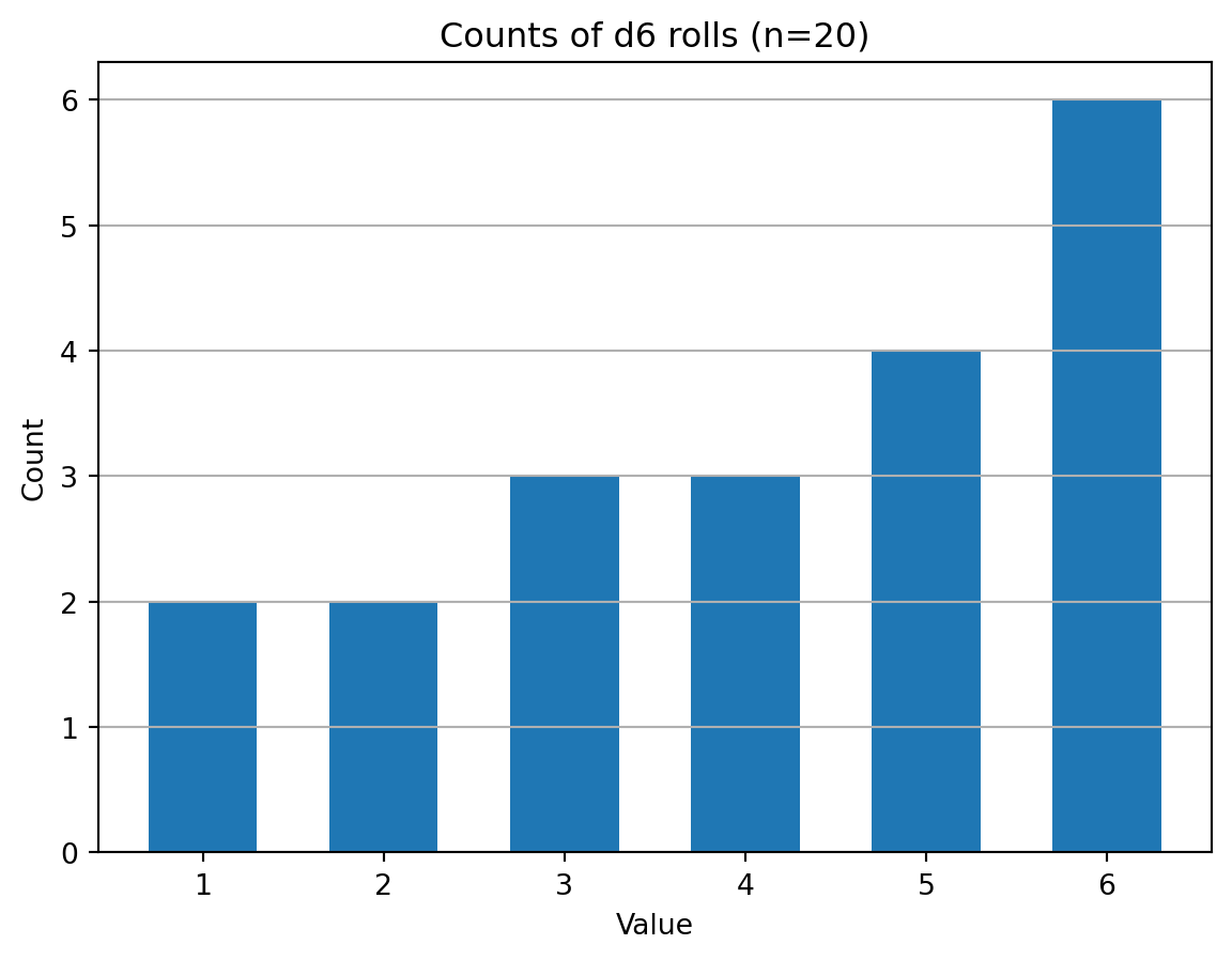

Increasing the sample size

results_200 = n_rolls_d6(200)
sorted_200 = sorted(results_200)
print(results_200)

[3, 5, 4, 1, 6, 4, 4, 5, 3, 1, 2, 5, 1, 6, 3, 1, 3, 2, 4, 5, 5, 6, 1, 6, 3, 4, 6, 6, 2, 5, 4, 2, 2, 5, 4, 4, 4, 1, 1, 2, 4, 2, 1, 3, 3, 6, 3, 4, 6, 4, 1, 1, 5, 1, 5, 3, 6, 1, 1, 4, 1, 5, 4, 1, 5, 6, 6, 4, 1, 3, 3, 4, 1, 5, 3, 4, 3, 1, 6, 6, 2, 4, 1, 6, 6, 2, 3, 6, 2, 6, 1, 6, 1, 5, 4, 5, 3, 2, 6, 3, 4, 3, 2, 5, 3, 5, 1, 6, 2, 5, 4, 4, 1, 6, 2, 4, 6, 1, 3, 4, 6, 6, 6, 6, 6, 4, 3, 4, 1, 2, 5, 3, 5, 5, 5, 2, 3, 5, 1, 5, 6, 3, 2, 5, 3, 1, 3, 5, 2, 2, 3, 3, 4, 1, 5, 1, 2, 5, 2, 1, 2, 3, 5, 2, 1, 5, 3, 1, 3, 5, 5, 2, 5, 2, 4, 4, 6, 4, 1, 3, 6, 5, 4, 3, 4, 2, 5, 2, 5, 6, 1, 5, 5, 4, 3, 6, 5, 1, 6, 1]

length_200 = len(results_200)
print("Number of rolls:", length_200)

Number of rolls: 200

Visual representation for the larger sample

results_200 = n_rolls_d6(200)

counts_200 = []
for value in range(1, 7):
    counts_200.append(results_200.count(value))

plt.figure()

plt.bar(range(1, 7), counts_200, width=0.6)

plt.title("Counts of d6 rolls (n=200)")
plt.xlabel("Value")
plt.ylabel("Count")

plt.grid(axis="y")
plt.xticks(range(1, 7))

plt.show()
plt.close()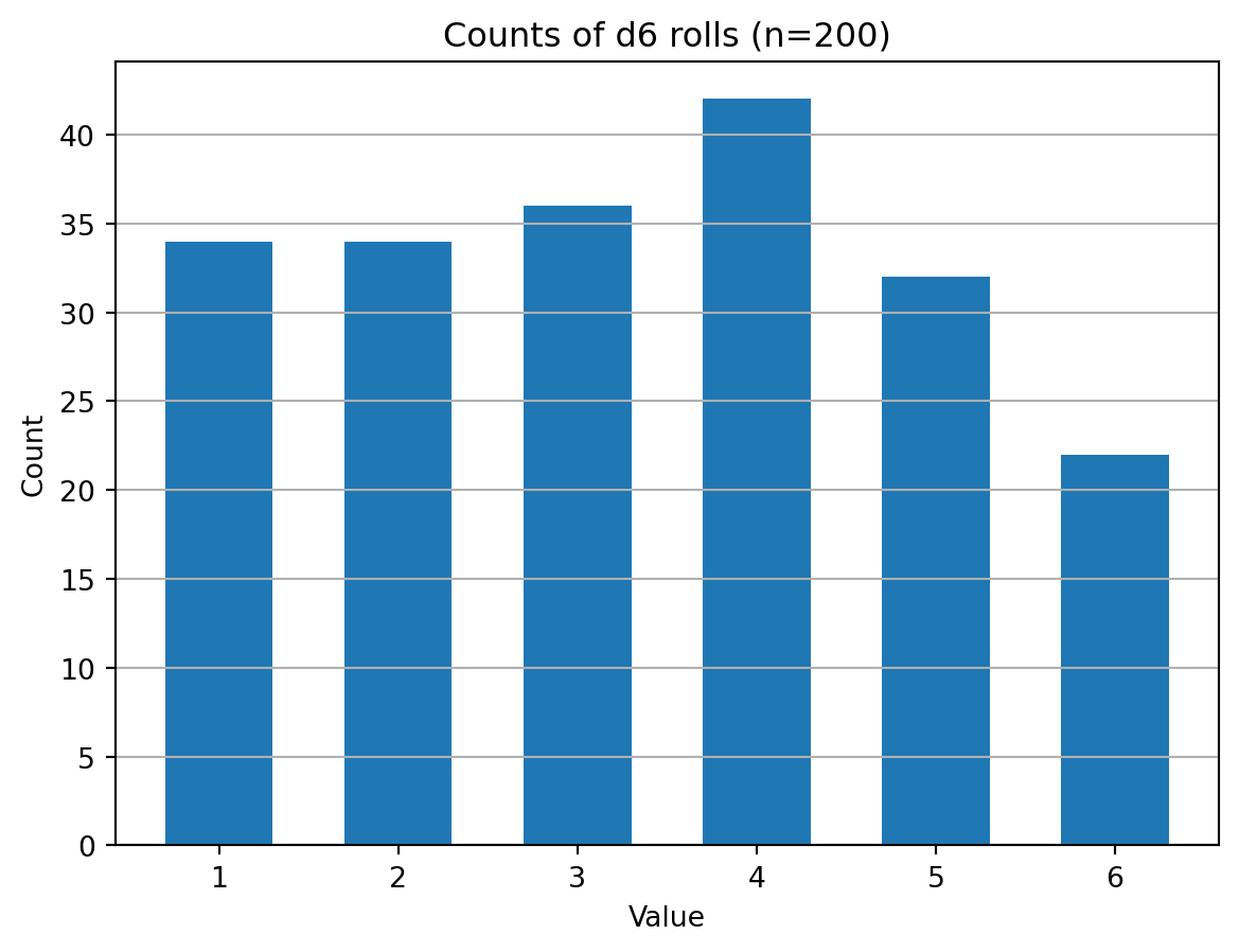

From counts to frequencies

Counts depend on how many d6 rolls we performed, so instead we focus on the frequency of each value v, defined as the number of times v appears, divided by the total number of rolls. Frequencies take values between 0 and 1, and can be interpreted as empirical probabilities.

print("Sample of 20:")
for value in range(1, 7):
    count = sorted_results.count(value)
    frequency = count / length_large
    print(value, frequency)

print("\nSample of 200:")
for value in range(1, 7):
    count = sorted_200.count(value)
    frequency = count / length_200
    print(value, frequency)

Sample of 20:
1 0.1
2 0.05
3 0.2
4 0.25
5 0.25
6 0.15

Sample of 200:
1 0.18
2 0.135
3 0.165
4 0.165
5 0.19
6 0.165

Side-by-side comparison, better

# theoretical (fair d6)
theoretical = [1/6 for _ in range(1, 7)]

# empirical n = 20
freq_20 = []
for value in range(1, 7):
    count_20 = sorted_results.count(value)
    freq_20.append(count_20 / length_large)

# empirical n = 200
freq_200 = []
for value in range(1, 7):
    count_200 = sorted_200.count(value)
    freq_200.append(count_200 / length_200)

print("value  prob    n=20         n=200")
for i in range(6): ## i+1 is one face of a d6
    print(
        i+1,
        theoretical[i],
        freq_20[i],
        freq_200[i]
    )

value  prob    n=20         n=200
1 0.16666666666666666 0.1 0.18
2 0.16666666666666666 0.05 0.135
3 0.16666666666666666 0.2 0.165
4 0.16666666666666666 0.25 0.165
5 0.16666666666666666 0.25 0.19
6 0.16666666666666666 0.15 0.165

Off-ramp: formatting and padding to create aligned tables

The following code improves readability of printed tables by aligning columns. This is not essential for the main logic, but can be useful for presentation.

def pad(text, width=12):
    return text + " " * (width - len(text))

print(
    pad("value")
    + pad("prob")
    + pad("n=20")
    + pad("n=200")
)

for i in range(6): ## i+1 is one face of a d6

    v = str(i + 1)

    t = f"{theoretical[i]:.3f}"
    p20 = f"{freq_20[i]:.3f}"
    p200 = f"{freq_200[i]:.3f}"

    print(
        pad(v)
        + pad(t)
        + pad(p20)
        + pad(p200)
    )

value       prob        n=20        n=200       
1           0.167       0.100       0.180       
2           0.167       0.050       0.135       
3           0.167       0.200       0.165       
4           0.167       0.250       0.165       
5           0.167       0.250       0.190       
6           0.167       0.150       0.165

Off-ramp: formatting via a dataframe

We can avoid manual formatting by using a dataframe.

import pandas as pd

values = list(range(1, 7))

df = pd.DataFrame({
    "value": values,
    "prob": theoretical,
    "n=20": freq_20,
    "n=200": freq_200
})

df = df.set_index("value")
df_rounded = df.round(3)
print(df_rounded)

        prob  n=20  n=200
value                    
1      0.167  0.10  0.180
2      0.167  0.05  0.135
3      0.167  0.20  0.165
4      0.167  0.25  0.165
5      0.167  0.25  0.190
6      0.167  0.15  0.165

repeating the experiment with more rolls

Let us add more samples. Note: the following code is very repetitive and not an example of good practice. If you find yourself copy-pasting large code blocks, there is usually a better way, typically writing a helper function.

results_200_b = n_rolls_d6(200)
sorted_200_b = sorted(results_200_b)
freq_200_b = []

for value in range(1, 7):
    count_200_b = sorted_200_b.count(value)
    freq_200_b.append(count_200_b / len(results_200_b))

results_2000 = n_rolls_d6(2000)
sorted_2000 = sorted(results_2000)
freq_2000 = []

for value in range(1, 7):
    count_2000 = sorted_2000.count(value)
    freq_2000.append(count_2000 / len(results_2000))
    
results_2000_b = n_rolls_d6(2000)
sorted_2000_b = sorted(results_2000_b)
freq_2000_b = []

for value in range(1, 7):
    count_2000_b = sorted_2000_b.count(value)
    freq_2000_b.append(count_2000_b / len(results_2000_b))

results_20000 = n_rolls_d6(20000)
sorted_20000 = sorted(results_20000)
freq_20000 = []

for value in range(1, 7):
    count_20000 = sorted_20000.count(value)
    freq_20000.append(count_20000 / len(results_20000))

results_20000_b = n_rolls_d6(20000)
sorted_20000_b = sorted(results_20000_b)
freq_20000_b = []

for value in range(1, 7):
    count_20000_b = sorted_20000_b.count(value)
    freq_20000_b.append(count_20000_b / len(results_20000_b))
        

df = pd.DataFrame({
    "value": values,
    "prob": theoretical,
    "n=20": freq_20,
    "n=200": freq_200,
    "200_b": freq_200_b,
    "n=2000": freq_2000,
    "2000_b": freq_2000_b,
    "n=20000": freq_20000,
    "20000_b": freq_20000_b,
})
df = df.set_index("value")
df_rounded = df.round(4)
print(df_rounded)

         prob  n=20  n=200  200_b  n=2000  2000_b  n=20000  20000_b
value                                                              
1      0.1667  0.10  0.180  0.230  0.1515  0.1770   0.1666   0.1707
2      0.1667  0.05  0.135  0.190  0.1785  0.1700   0.1656   0.1648
3      0.1667  0.20  0.165  0.180  0.1640  0.1605   0.1704   0.1655
4      0.1667  0.25  0.165  0.145  0.1630  0.1710   0.1648   0.1674
5      0.1667  0.25  0.190  0.115  0.1605  0.1590   0.1648   0.1645
6      0.1667  0.15  0.165  0.140  0.1825  0.1625   0.1679   0.1672

repeating the experiment with more rolls (compact code version)

A more compact, less error-prone version of the same code:

values = list(range(1, 7))
# theoretical (fair d6)
theoretical = [1/6 for _ in range(1, 7)]

def compute_frequencies(n):
    results = n_rolls_d6(n)
    frequencies = []
    for value in range(1, 7):
        count = results.count(value)
        frequencies.append(count / len(results))
    return frequencies

df_series={
    "value": values,
    "prob": theoretical,}
    
series_names_list=[]
for n in [20,200,200,2000,2000,20000,20000]:
    series_name="n="+str(n) ## string concatenation
    if series_name in series_names_list:
        series_name+="_"  ## if two samples have the same size
    series_names_list.append(series_name)
    df_series[series_name]=compute_frequencies(n)
df = pd.DataFrame(df_series)
df = df.set_index("value")
df_rounded = df.round(4)

print(df_rounded)

         prob  n=20  n=200  n=200_  n=2000  n=2000_  n=20000  n=20000_
value                                                                 
1      0.1667  0.10  0.185   0.180  0.1555   0.1665   0.1700    0.1684
2      0.1667  0.15  0.165   0.210  0.1585   0.1835   0.1676    0.1670
3      0.1667  0.20  0.150   0.185  0.1700   0.1570   0.1690    0.1696
4      0.1667  0.15  0.170   0.165  0.1770   0.1570   0.1599    0.1688
5      0.1667  0.10  0.165   0.145  0.1735   0.1735   0.1636    0.1648
6      0.1667  0.30  0.165   0.115  0.1655   0.1625   0.1700    0.1614

Visualizations using frequencies and sample size

In The Effect

distribution https://theeffectbook.net/ch-DescribingVariables.html#the-distribution
theoretical distribution https://theeffectbook.net/ch-DescribingVariables.html#theoretical-distributions
sampling variation https://theeffectbook.net/ch-Simulation.html#the-anatomy-of-a-simulation
histogram https://theeffectbook.net/ch-DescribingVariables.html#the-distribution

The previous visualizations used counts. Let us now visualize frequencies.

plt.figure()

plt.bar(range(1, 7), freq_200, width=0.6)

plt.axhline(1/6, color="black", linestyle="--")  # theoretical frequency

plt.title("Frequencies of d6 rolls (n=200)")
plt.xlabel("Value")
plt.ylabel("Frequency")


plt.xticks(range(1, 7))

# y tickmarks at multiples of 1/24
plt.yticks([i/24 for i in range(25)])  ## list comprehension

## Restrict span of the vertical axis
max_height = max(freq_200)
y_max = 1.15 * max_height

plt.ylim(0, y_max)

plt.grid(axis="y")

plt.show()
plt.close()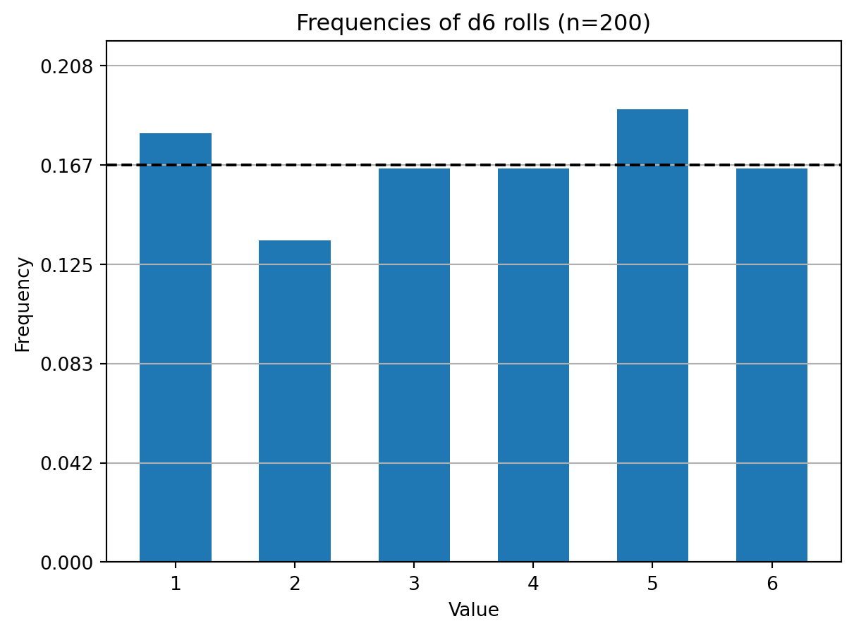

Again, for the larger sample.

plt.figure()

plt.bar(range(1, 7), freq_20000, width=0.6)

plt.axhline(1/6, color="black", linestyle="--")  # theoretical frequency

plt.title("Frequencies of d6 rolls (n=20000)")
plt.xlabel("Value")
plt.ylabel("Frequency")

plt.grid(axis="y")
plt.xticks(range(1, 7))

# y tickmarks at multiples of 1/24
plt.yticks([i/24 for i in range(25)])

## Restrict span of the vertical axis
max_height = max(freq_20000)
y_max = 1.15 * max_height

plt.ylim(0, y_max)
plt.show()
plt.close()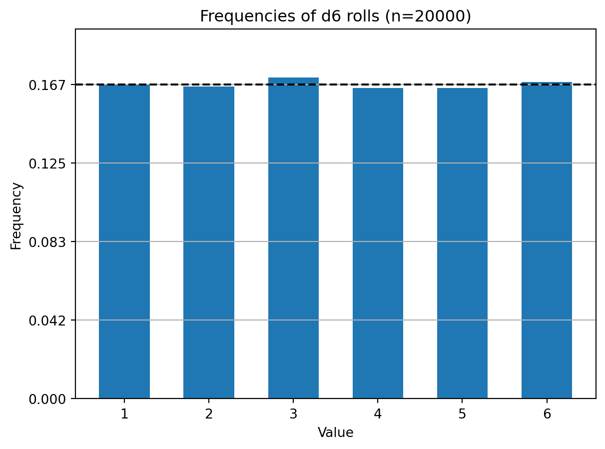

Across repeated samples:

Frequencies vary from sample to sample.
For large samples, frequencies are close to the theoretical probability \(\frac{1}{6}\).
Sample frequencies converge toward their theoretical probability as the sample size grows, this is an instance of the law of large numbers.

Descriptive statistics

We now move from looking at raw data and frequencies to summarizing data. Some vocabulary:

A random variable is a numerical quantity generated by a random process (for example, one roll of a d6).

A realization or observation is a value that the random variable actually takes when executing the random process (for example, observing a 4 upon rolling a d6).

A sample or data series is a finite list of realizations. The number of observations is the sample size.

A statistic is a number computed from a data series to quantify one of its features.

We will construct a data series where each observation is the sum of four d6 rolls (4d6).

import random

def roll_4d6():
    total = 0
    for i in range(4):
        total += random.randint(1, 6)
    return total

def generate_4d6_series(n_observations):
    results = []
    for i in range(n_observations):
        results.append(roll_4d6())
    return results

Note: The function generate_4d6_series repeatedly calls the function roll_4d6.

n_observations_4d6 = 800

rolls_4d6 = generate_4d6_series(n_observations_4d6)

print(rolls_4d6[:10])

[21, 17, 15, 12, 14, 19, 12, 22, 15, 11]

It’s always a good idea to print a small amount of your dataset and/or visually inspect it. It’s also a good idea to try to visualize your variables, typically with histograms or summary tables.

frequencies_4d6 = [
    rolls_4d6.count(total)
    for total in range(4, 25)
]

plt.bar(range(4, 25), frequencies_4d6)
plt.xlabel("Sum of four d6 rolls")
plt.ylabel("Frequency")
plt.xticks(range(4, 25))
plt.show()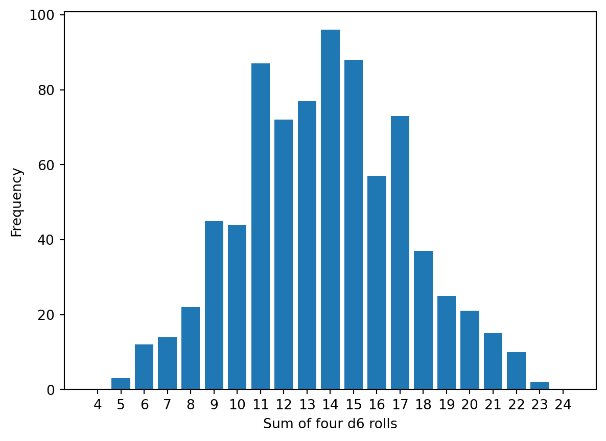

Mean

mean_4d6 = sum(rolls_4d6) / n_observations_4d6
print(mean_4d6)

13.73375

Minimum and maximum

print(min(rolls_4d6), max(rolls_4d6))

5 23

Median

sorted_4d6 = sorted(rolls_4d6)

median_4d6 = sorted_4d6[n_observations_4d6 // 2]

print(median_4d6)

Quantiles and quartiles

q25_4d6 = sorted_4d6[n_observations_4d6 // 4]
q50_4d6 = sorted_4d6[n_observations_4d6 // 2]
q75_4d6 = sorted_4d6[(3 * n_observations_4d6) // 4]

print(q25_4d6, q50_4d6, q75_4d6)

iqr_4d6 = q75_4d6 - q25_4d6
print(iqr_4d6)

11 14 16
5

Variance and standard deviation

sq_diffs_4d6 = []

for value in rolls_4d6:
    diff = value - mean_4d6
    sq_diffs_4d6.append(diff**2)

variance_4d6 = sum(sq_diffs_4d6) / (n_observations_4d6-1)
## we divide by (n-1) because <stats reasons>, 
## see a stats textbook on "sample variance"
std_4d6 = variance_4d6 ** 0.5

print(variance_4d6)
print(std_4d6)

12.380836983729662
3.5186413548029676

Summary and .describe()

In The Effect

summarizing https://theeffectbook.net/ch-DescribingVariables.html#summarizing-the-distribution
mean https://theeffectbook.net/ch-DescribingVariables.html#summarizing-the-distribution
median https://theeffectbook.net/ch-DescribingVariables.html#summarizing-the-distribution
variance https://theeffectbook.net/ch-DescribingVariables.html#summarizing-the-distribution
standard deviation https://theeffectbook.net/ch-DescribingVariables.html#summarizing-the-distribution
range https://theeffectbook.net/ch-DescribingVariables.html#summarizing-the-distribution
distribution https://theeffectbook.net/ch-DescribingVariables.html#the-distribution
variable https://theeffectbook.net/ch-DescribingVariables.html#descriptions-of-variables
observations https://theeffectbook.net/ch-DescribingVariables.html#summarizing-the-distribution

We have now introduced several statistics used to describe a data series. - A measure of location summarizes central tendency (mean, median, mode) - A measure of dispersion summarizes variability (variance, standard deviation, interquartile range)

These statistics can be computed manually, as we have done so far. They can also be obtained automatically using the .describe() method from the pandas library, which returns a standard set of summary statistics for each variable in a dataframe.

import pandas as pd

df_4d6 = pd.DataFrame({
    "rolls_4d6": rolls_4d6
})

print("d6 summary:")
print(df_4d6.describe())

d6 summary:
        rolls_4d6
count  800.000000
mean    13.733750
std      3.518641
min      5.000000
25%     11.000000
50%     14.000000
75%     16.000000
max     23.000000

Rigged d6 vs fair d6: construction

In The Effect

hypothesis https://theeffectbook.net/ch-ResearchQuestions.html#what-is-a-research-question
hypothesis testing https://theeffectbook.net/ch-StatisticalAdjustment.html#hypothesis-testing-in-ols
null hypothesis https://theeffectbook.net/ch-DescribingVariables.html#theoretical-distributions
false positives https://theeffectbook.net/ch-ResearchQuestions.html#why-start-with-a-question
p-value https://theeffectbook.net/ch-StatisticalAdjustment.html#hypothesis-testing-in-ols
significance https://theeffectbook.net/ch-StatisticalAdjustment.html#regression-tables-and-model-fit-statistics
distribution https://theeffectbook.net/ch-DescribingVariables.html#the-distribution
conditional distribution https://theeffectbook.net/ch-DescribingRelationships.html#conditional-distributions
theoretical distribution https://theeffectbook.net/ch-DescribingVariables.html#theoretical-distributions
mean https://theeffectbook.net/ch-DescribingVariables.html#summarizing-the-distribution
sampling variation https://theeffectbook.net/ch-Simulation.html#the-anatomy-of-a-simulation

We now move to hypothesis testing. So far, we have described data generated by a known data generating process. We now reverse the perspective: we observe data and try to infer the data generating process that produced it.

First, we need to define what a rigged d6 is and implement it in code.

We will construct both a fair d6 and a rigged d6 using the same interval-based method, making their probability distributions easy to compare.

import random
import matplotlib.pyplot as plt
import pandas as pd

random.seed(1236)

interval_widths_fair = [12, 12, 12, 12, 12, 12]
interval_widths_rigged = [10, 8, 12, 12, 16, 14]

assert sum(interval_widths_fair) == 72
assert sum(interval_widths_rigged) == 72

thresholds_fair = []
running_total = 0

for interval_width in interval_widths_fair:
    running_total += interval_width
    thresholds_fair.append(running_total)

thresholds_rigged = []
running_total = 0

for interval_width in interval_widths_rigged:
    running_total += interval_width
    thresholds_rigged.append(running_total)

probabilities_fair = []

for interval_width in interval_widths_fair:
    probabilities_fair.append(interval_width / 72)

probabilities_rigged = []

for interval_width in interval_widths_rigged:
    probabilities_rigged.append(interval_width / 72)

def roll_fair_d6():

    draw = random.randint(1, 72)

    for face, threshold in enumerate(thresholds_fair, start=1):
        if draw <= threshold:
            return face

def roll_rigged_d6():

    draw = random.randint(1, 72)

    for face, threshold in enumerate(thresholds_rigged, start=1):
        if draw <= threshold:
            return face

Rigged d6 vs fair d6: visualizing the mapping

import matplotlib.pyplot as plt

plt.figure(figsize=(10, 3))

plt.hlines(2, 1, 72)

for threshold in thresholds_fair:
    plt.vlines(threshold, 2, 2.6, color="blue")

for threshold in thresholds_rigged:
    plt.vlines(threshold, 1.4, 2, color="red")

all_ticks = sorted(set([1] + thresholds_fair + thresholds_rigged))

start = 1

for face, interval_width in enumerate(interval_widths_fair, start=1):
    midpoint = start + (interval_width - 1) / 2
    plt.text(midpoint, 2.2, str(face), color="blue", ha="center", fontsize=12)
    start += interval_width

start = 1

for face, interval_width in enumerate(interval_widths_rigged, start=1):
    midpoint = start + (interval_width - 1) / 2
    plt.text(midpoint, 1.6, str(face), color="red", ha="center", fontsize=12)
    start += interval_width

plt.xlim(1, 72)
plt.ylim(1.4, 2.6)

plt.xticks(all_ticks)
plt.yticks([])

ax = plt.gca()
ax_top = ax.secondary_xaxis("top")

ax_top.set_xticks(all_ticks)
ax_top.set_xticklabels(all_ticks)

plt.grid(axis="x", alpha=0.3)

plt.title("Mapping from [1,72] to d6 outcomes")
plt.xlabel("Integer draw")

plt.show()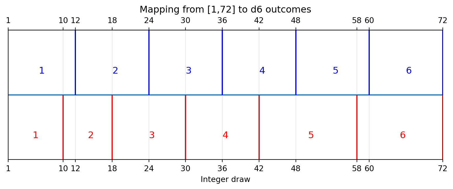

Blue labels correspond to the fair d6 mapping.

Red labels correspond to the rigged d6 mapping.

fair d6: each face receives 12 integers and therefore occurs with probability (12/72 = 1/6)
rigged d6: each face receives a different number of integers and therefore occurs with a different probability

The probability distributions implied by the two data generating processes are:

df_probabilities = pd.DataFrame({
    "face": [1, 2, 3, 4, 5, 6],
    "probabilities_fair": probabilities_fair,
    "probabilities_rigged": probabilities_rigged
})

print(df_probabilities.round(3))

   face  probabilities_fair  probabilities_rigged
0     1               0.167                 0.139
1     2               0.167                 0.111
2     3               0.167                 0.167
3     4               0.167                 0.167
4     5               0.167                 0.222
5     6               0.167                 0.194

Empirical comparison and varying the sample size

We now generate samples from each d6 and compare their empirical frequencies with the corresponding theoretical probabilities.

sample_sizes = [20, 200, 2000, 20000]

results_all = []
max_height = 0

for sample_size in sample_sizes:

    sample_fair = []

    for roll_number in range(sample_size):
        sample_fair.append(roll_fair_d6())

    sample_rigged = []

    for roll_number in range(sample_size):
        sample_rigged.append(roll_rigged_d6())

    freqs_fair = []

    for face in range(1, 7):
        freqs_fair.append(
            sample_fair.count(face) / sample_size
        )

    freqs_rigged = []

    for face in range(1, 7):
        freqs_rigged.append(
            sample_rigged.count(face) / sample_size
        )

    results_all.append(
        (
            sample_size,
            freqs_fair,
            freqs_rigged
        )
    )

    max_height = max(
        max_height,
        max(freqs_fair),
        max(freqs_rigged)
    )

y_max = 1.15 * max_height

step = 1 / 36
yticks = []
current = 0

while current <= y_max:
    yticks.append(current)
    current += step

fig, axes = plt.subplots(4, 2, figsize=(8, 16))

for row, (sample_size, freqs_fair, freqs_rigged) in enumerate(results_all):

    axes[row, 0].bar(range(1, 7), freqs_fair, color="blue")

    for face, probability in enumerate(probabilities_fair, start=1):
        axes[row, 0].hlines(
            probability,
            face - 0.3,
            face + 0.3,
            linestyles="--",
            color="black"
        )

    axes[row, 0].set_title(f"Fair d6 (n={sample_size})")
    axes[row, 0].grid(axis="y", alpha=0.3)

    axes[row, 1].bar(range(1, 7), freqs_rigged, color="red")

    for face, probability in enumerate(probabilities_rigged, start=1):
        axes[row, 1].hlines(
            probability,
            face - 0.3,
            face + 0.3,
            linestyles="--",
            color="black"
        )

    axes[row, 1].set_title(f"Rigged d6 (n={sample_size})")
    axes[row, 1].grid(axis="y", alpha=0.3)

    for col in [0, 1]:
        axes[row, col].set_ylim(0, y_max)
        axes[row, col].set_yticks(yticks)

plt.tight_layout()
plt.show()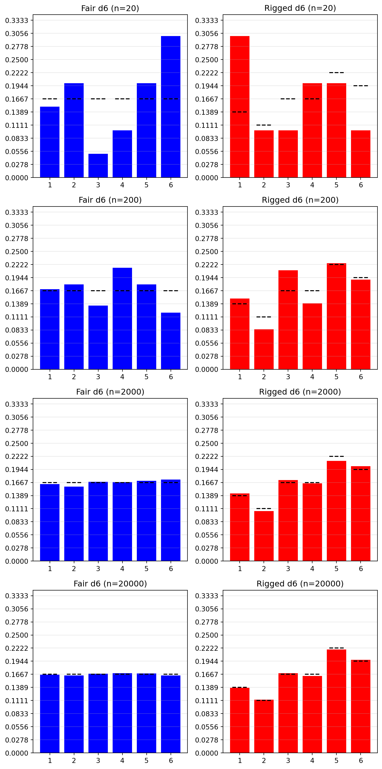

Across repeated samples:

Frequencies vary from sample to sample.
For large samples, frequencies are close to the theoretical probability for each face.

Differences across samples are an example of sampling variation.

For large samples, empirical frequencies tend to become close to the corresponding theoretical probabilities. This is another illustration of the Law of Large Numbers.

Testing whether a given d6 is fair

We now move from describing samples to making decisions from them. Suppose we are given a sample of n=50 rolls from a d6 with unknown type. A natural question is: Based on the evidence, is this d6 fair, or is it rigged?

The code below recreates this uncertainty by randomly deciding whether each sample comes from the fair d6 or the rigged d6. You can run it multiple times to generate a new collection of unknown samples.

sample_size = 50
prob_rigged = 0.48

fig, axes = plt.subplots(3, 2, figsize=(8, 12))

fair_indices = []  # store outcomes for printing later
rigged_indices = []  # store outcomes for printing later

for i in range(6): ## draw 6 samples (6 simulations)

    is_rigged = random.random() < prob_rigged

    if is_rigged:

        sample_unknown = []

        for roll_number in range(sample_size):
            sample_unknown.append(roll_rigged_d6())

        rigged_indices.append(i)

    else:

        sample_unknown = []

        for roll_number in range(sample_size):
            sample_unknown.append(roll_fair_d6())

        fair_indices.append(i)

    freqs_unknown = []

    for face in range(1, 7):
        freqs_unknown.append(
            sample_unknown.count(face) / sample_size
        )

    row = i // 2
    col = i % 2
    ax = axes[row, col]

    ax.bar(range(1, 7), freqs_unknown, width=0.6, color="gray", alpha=0.5)

    for x, y in enumerate(probabilities_fair, start=1):
        ax.hlines(y, x-0.3, x+0.3, linestyles="--", color="blue")

    for x, y in enumerate(probabilities_rigged, start=1):
        ax.hlines(y, x-0.3, x+0.3, linestyles=":", color="red")

    ax.set_title(f"Unknown_{i} d6 (n={sample_size})")
    ax.set_xlabel("Value")
    ax.set_ylabel("Frequency")

    ax.grid(axis="y")
    ax.set_xticks(range(1, 7))

    # y tickmarks
    ax.set_yticks([i/36 for i in range(37)])

    # restrict vertical axis
    max_height = max(freqs_unknown)
    y_max = 1.2 * max_height
    ax.set_ylim(0, y_max)

plt.tight_layout()
plt.show()

# print results after all plots
print("The fair d6 types were", fair_indices, ". The rigged d6 types were", rigged_indices)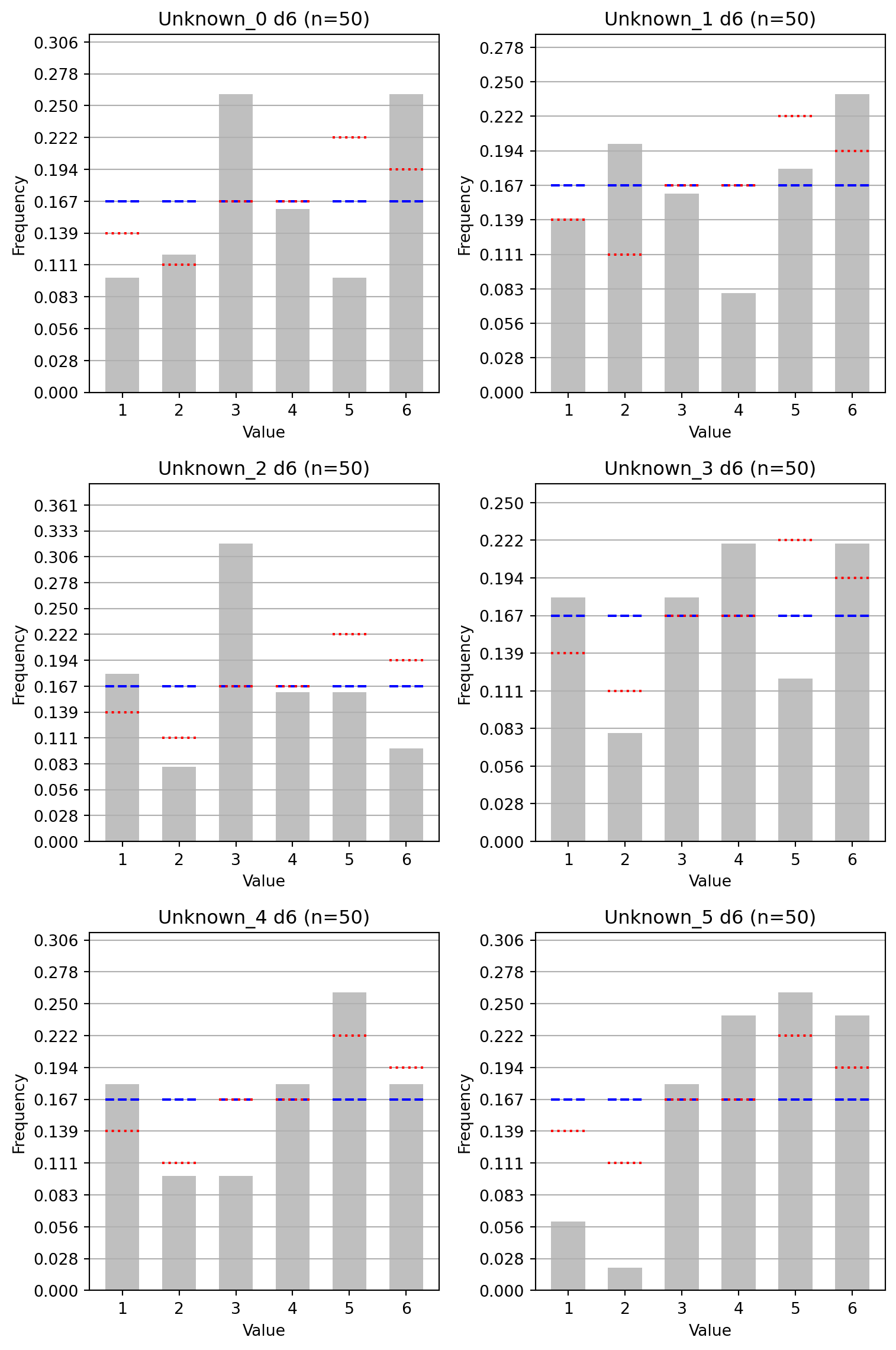

The fair d6 types were [0, 3] . The rigged d6 types were [1, 2, 4, 5]

We know that the histogram from the rigged d6 is “lopsided”, but how lopsided is too lopsided? We need a systematic way to decide. Staring at histograms and going with visual intuition is not transparent or reproducible. Instead, we introduce two tools:

a test statistic: a number computed from the sample
a decision rule: a rule telling us when that number is “too extreme”

A test statistic summarizes the information contained in the sample (the six empirical frequencies) into a single number. We should typically get higher sample means from the rigged d6, so we will use the sample mean as a test statistic to detect a rigged d6. The sample mean is not the best available test statistic, we will return to that point later.

values = [1,2,3,4,5,6]

expected_fair = sum(v*p for v,p in zip(values,probabilities_fair))
expected_rigged = sum(v*p for v,p in zip(values,probabilities_rigged))

print(f"Expected sample mean (fair d6): {expected_fair:.3f}")
print(f"Expected sample mean (rigged d6): {expected_rigged:.3f}")

Expected sample mean (fair d6): 3.500
Expected sample mean (rigged d6): 3.806

import matplotlib.pyplot as plt

sample_size = 50
n_simulations = 400

means_fair = []
means_rigged = []

for _ in range(n_simulations):
    sample_fair = [roll_fair_d6() for _ in range(sample_size)]
    sample_rigged = [roll_rigged_d6() for _ in range(sample_size)]
    
    means_fair.append(sum(sample_fair) / sample_size)
    means_rigged.append(sum(sample_rigged) / sample_size)

# build discrete frequencies
x_vals = sorted(set(means_fair + means_rigged))

freqs_fair = []
freqs_rigged = []

for x in x_vals:
    freqs_fair.append(means_fair.count(x) / n_simulations)
    freqs_rigged.append(means_rigged.count(x) / n_simulations)

bar_width = 1 / sample_size

plt.figure(figsize=(8,5))

plt.bar(x_vals, freqs_fair, width=bar_width, alpha=0.6, color="darkblue", label="fair d6")
plt.bar(x_vals, freqs_rigged, width=bar_width, alpha=0.6, color="darkred", label="rigged d6")

plt.axvline(expected_fair, color="black", linestyle="--")

plt.xlabel(f"sample mean (n={sample_size})")
plt.ylabel("frequency")
plt.title(f"Sample mean (n={sample_size}), across {n_simulations} simulations")
plt.legend()

plt.grid(alpha=0.3)

plt.show()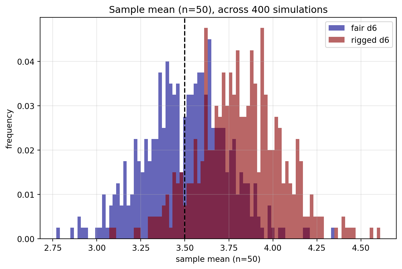

The two distributions are centered at different values: high sample means are more likely to happen with a rigged d6 than with a fair d6. However, the two distributions overlap: some rigged d6 samples have a lower sample mean than some fair d6 samples. So the sample mean is an imperfect statistic and we will never be able to guarantee that we can detect a rigged d6 using only a sample of 50 rolls. In general, hypothesis testing does not produce definitive answers, instead it aims to quantify uncertainty.

Hypotheses, decision rule, type I error and type II error

A statistical hypothesis test is a procedure to formally decide whether there is enough information in the data available to reject a particular statement known as the null hypothesis. In our application,

null hypothesis \(H_0\): the d6 is fair
alternative hypothesis \(H_{1}\): the d6 is rigged

Decision rule: If the null hypothesis is correct, the d6 is fair, and the sample mean should be close to 3.5. If the sample mean is sufficiently far from 3.5, we reject the null hypothesis. The challenge is to formally and transparently decide on what “close to” and “sufficiently far from” mean for our application.

Any decision rule gives rise to two types of errors: A type I error (incorrectly reject) corresponds to rejecting \(H_0\) when the d6 is in fact fair. A type II error (failure to correctly reject) corresponds to failing to reject \(H_0\) when the d6 is in fact rigged.

Note that the statistical hypothesis test framework embeds an asymmetry: we never accept the null hypothesis, we simply reject or fail to reject it. See https://decodingstatistics.substack.com/p/why-statisticians-say-fail-to-reject-instead-of-accept-the-null.

Distribution of the sample mean under \(H_0\)

sample_size = 50
n_simulations = 3000

means_H0 = [
    sum(roll_fair_d6() for _ in range(sample_size))/sample_size
    for _ in range(n_simulations)
]

x_vals = sorted(set(means_H0))
freqs = [means_H0.count(x)/n_simulations for x in x_vals]

bar_width = 1/sample_size

plt.figure(figsize=(8,5))
plt.bar(x_vals, freqs, width=bar_width, color="blue")

plt.axvline(expected_fair, linestyle="--")
plt.title("Sample mean under H0")
plt.grid(alpha=0.3)
plt.show()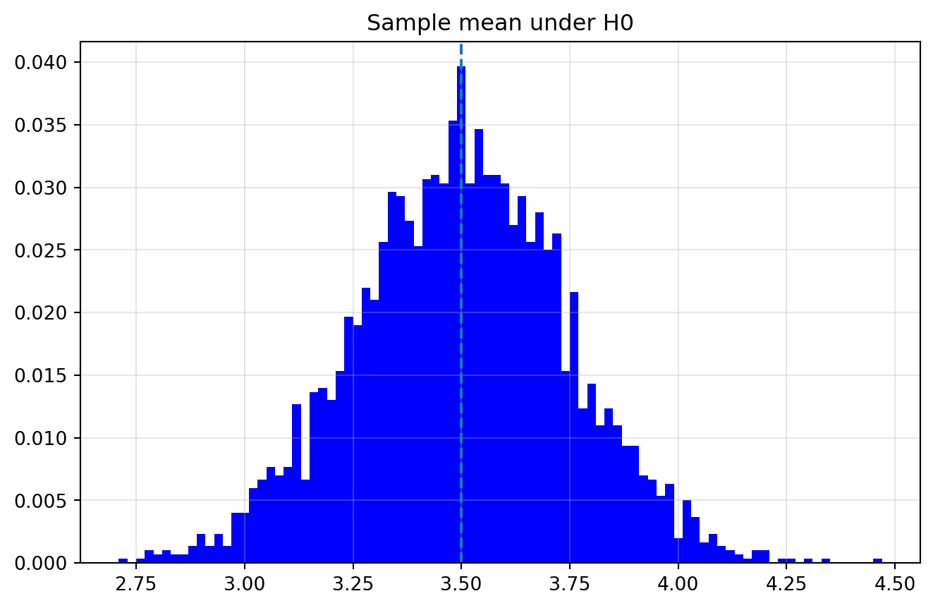

Decision rule and p-values

In hypothesis testing, we first choose a target frequency of Type I errors.

We then reject the null hypothesis for sufficiently extreme values of the test statistic.

alpha = 0.10

def jitter(x, scale):
    return x + random.uniform(-scale, scale)

means_H0_j = [jitter(m, 1e-6) for m in means_H0]
cutoff_means_H0_j_10pct = sorted(means_H0_j)[int((1-alpha) * n_simulations)]

print(f"Decision rule: reject H0 if sample mean ≥ {cutoff_means_H0_j_10pct:.3f}")

Decision rule: reject H0 if sample mean ≥ 3.820

The same decision rule can be expressed using p-values: for a realized value of the test statistic T, the p-value of T is the probability (under \(H_0\)) of observing a value at least as extreme as T. Small p-values correspond to realizations which are unlikely under \(H_0\), large p-values correspond to realizations which are likely under \(H_0\).

The realized sample mean T is in the top 10% of possible realizations under \(H_0\).

is equivalent to

The realized sample mean T has a p-value (under \(H_0\)) of 0.1 or less.

Visualizing the rejection region

x_fail = []
y_fail = []
x_reject = []
y_reject = []

for x, y in zip(x_vals, freqs):
    if x < cutoff_means_H0_j_10pct:
        x_fail.append(x)
        y_fail.append(y)
    else:
        x_reject.append(x)
        y_reject.append(y)

plt.figure(figsize=(8,5))
plt.bar(x_fail, y_fail, width=bar_width, color="blue")
plt.bar(x_reject, y_reject, width=bar_width, color="red")

plt.axvline(cutoff_means_H0_j_10pct, linestyle=":", label="cutoff (90th pctile)", color="black")

plt.title("Decision rule: reject iff sample mean is in the top 10%")
plt.xlabel(f"sample mean (n={sample_size})")
plt.ylabel("frequency")

plt.legend()
plt.grid(alpha=0.3)
plt.show()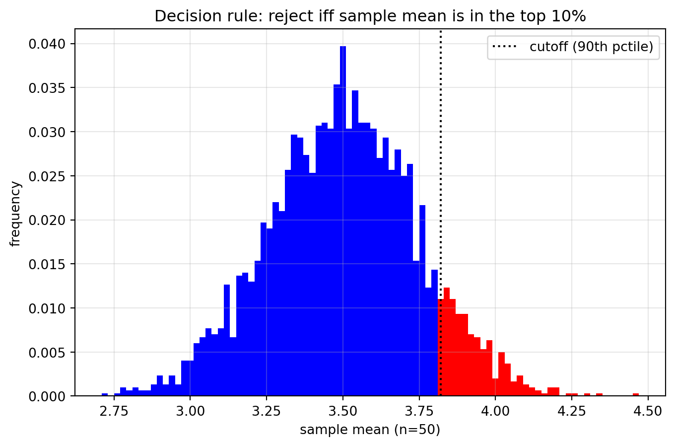

Blue values correspond to realizations for which we fail to reject \(H_0\).
Red values correspond to realizations for which we reject \(H_0\).

Simulating repeated tests

In each simulation, a hypothetical d6-making machine produces a d6, which is: - a fair d6 with probability prob_fair
- a rigged d6 with probability prob_rigged

the d6 inspector receives the newly-produced d6
rolls it sample_size times
computes the sample mean
compares it to the cutoff (90th percentile of sample mean)
rejects \(H_0\) iff the sample mean exceeds the cutoff

We could equivalently reformulate the inspector’s decision in terms of p-values: 4’. computes the p-value of the sample mean 5’. rejects \(H_0\) iff the p-value is 0.1 or less

random.seed(999)

min_trials = 20
max_trials = 60
prob_rigged = 0.30
prob_fair = 1 - prob_rigged

def compute_p_value(stat, reference):
    return sum(x >= stat for x in reference) / len(reference)

print(f"Decision rule: reject H0 iff the mean exceeds {cutoff_means_H0_j_10pct:.3f}")

examples = {
    "Type I": None,
    "Type II": None,
    "correct_reject": None,
    "correct_fail": None
}

t = 0

while True:

    is_rigged = random.random() < prob_rigged
    generator = roll_rigged_d6 if is_rigged else roll_fair_d6

    sample = [generator() for _ in range(sample_size)]
    m = sum(sample) / sample_size
    m_j = jitter(m, 1e-6)

    p_value = compute_p_value(m, means_H0)
    reject = m_j >= cutoff_means_H0_j_10pct

    if is_rigged and reject:
        outcome = "correctly reject H0 while d6 is rigged"
        key = "correct_reject"
    elif is_rigged:
        outcome = "Type II; fail to reject H0 while d6 is rigged"
        key = "Type II"
    elif reject:
        outcome = "Type I; incorrectly reject H0 while d6 is fair"
        key = "Type I"
    else:
        outcome = "correctly fail to reject H0 while d6 is fair"
        key = "correct_fail"

    # store first occurrence
    if examples[key] is None:
        examples[key] = {
            "trial": t,
            "mean": m,
            "p": p_value,
            "group": "reject" if key in ["Type I", "correct_reject"] else "fail",
            "is_rigged": is_rigged,
            "outcome": outcome
        }

    print(f"Trial {t:02d} | {'rigged' if is_rigged else 'fair':6s} | mean={m_j:.3f} | p-value={p_value:.3f} | {outcome}")

    t += 1
    # stopping conditions
    all_types_found = all(v is not None for v in examples.values())

    if (t >= min_trials and all_types_found) or t >= max_trials:
        break

Decision rule: reject H0 iff the mean exceeds 3.820
Trial 00 | fair   | mean=3.300 | p-value=0.808 | correctly fail to reject H0 while d6 is fair
Trial 01 | rigged | mean=3.880 | p-value=0.066 | correctly reject H0 while d6 is rigged
Trial 02 | fair   | mean=3.700 | p-value=0.215 | correctly fail to reject H0 while d6 is fair
Trial 03 | rigged | mean=3.560 | p-value=0.417 | Type II; fail to reject H0 while d6 is rigged
Trial 04 | fair   | mean=3.600 | p-value=0.355 | correctly fail to reject H0 while d6 is fair
Trial 05 | rigged | mean=3.940 | p-value=0.040 | correctly reject H0 while d6 is rigged
Trial 06 | fair   | mean=3.500 | p-value=0.522 | correctly fail to reject H0 while d6 is fair
Trial 07 | fair   | mean=3.360 | p-value=0.731 | correctly fail to reject H0 while d6 is fair
Trial 08 | fair   | mean=3.080 | p-value=0.958 | correctly fail to reject H0 while d6 is fair
Trial 09 | fair   | mean=3.300 | p-value=0.808 | correctly fail to reject H0 while d6 is fair
Trial 10 | rigged | mean=3.920 | p-value=0.047 | correctly reject H0 while d6 is rigged
Trial 11 | fair   | mean=3.300 | p-value=0.808 | correctly fail to reject H0 while d6 is fair
Trial 12 | rigged | mean=3.560 | p-value=0.417 | Type II; fail to reject H0 while d6 is rigged
Trial 13 | fair   | mean=3.860 | p-value=0.077 | Type I; incorrectly reject H0 while d6 is fair
Trial 14 | fair   | mean=3.420 | p-value=0.649 | correctly fail to reject H0 while d6 is fair
Trial 15 | fair   | mean=3.360 | p-value=0.731 | correctly fail to reject H0 while d6 is fair
Trial 16 | fair   | mean=3.440 | p-value=0.619 | correctly fail to reject H0 while d6 is fair
Trial 17 | rigged | mean=3.680 | p-value=0.243 | Type II; fail to reject H0 while d6 is rigged
Trial 18 | fair   | mean=3.500 | p-value=0.522 | correctly fail to reject H0 while d6 is fair
Trial 19 | rigged | mean=4.220 | p-value=0.002 | correctly reject H0 while d6 is rigged

We now place one example of each outcome on the rejection-region figure.

plt.figure(figsize=(8,5))

plt.bar(x_fail, y_fail, width=bar_width, color="blue")
plt.bar(x_reject, y_reject, width=bar_width, color="red")

plt.axvline(cutoff_means_H0_j_10pct, linestyle=":", label="cutoff (90th pctile)")

# simple color map (local, readable)
color_map = {
    "Type I": "black",
    "Type II": "beige",
    "correct_reject": "purple",
    "correct_fail": "pink"
}

# manual y-placement: different across AND within groups
y_positions = {
    "Type I": 0.95,
    "correct_reject": 0.87,
    "Type II": 0.07,
    "correct_fail": 0.15
}

# manual y-align: different in reject
y_align = {
    "Type I": "left",
    "correct_reject": "left",
    "Type II": "center",
    "correct_fail": "center"
}

# plotting
for key, value in examples.items():
    if value is None:
        continue

    x_val = value["mean"]
    trial_id = value["trial"]
    p_val = value["p"]

    color = color_map[key]
    y_text = max(freqs) * y_positions[key]

    # line ends just below text
    y_line = y_text * 0.97

    ha = y_align[key]

    # draw truncated line
    plt.vlines(x_val, 0, y_line, color=color)

    # label close to line (not floating too high)
    plt.text(
        x_val,
        y_text,
        f"T{trial_id:02d} p={p_val:.3f}",
        ha=ha,
        color=color
    )

plt.title("Rejection region with selected trials")
plt.xlabel(f"sample mean (n={sample_size})")
plt.ylabel("frequency")

plt.grid(alpha=0.3)
plt.show()

print("Trials displayed on the figure:")
for key, value in examples.items():
    print(f'T{value["trial"]:02d} | {"rigged" if value["is_rigged"] else "fair":6s} | mean={value["mean"]:.3f} | p-value={value["p"]:.3f} | {key}')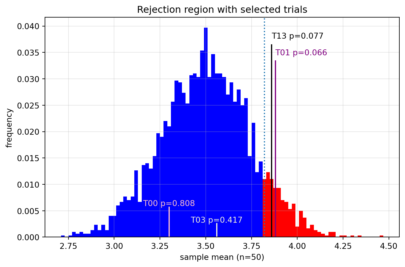

Trials displayed on the figure:
T13 | fair   | mean=3.860 | p-value=0.077 | Type I
T03 | rigged | mean=3.560 | p-value=0.417 | Type II
T01 | rigged | mean=3.880 | p-value=0.066 | correct_reject
T00 | fair   | mean=3.300 | p-value=0.808 | correct_fail

Each point illustrates:

its position relative to the cutoff
the corresponding p-value
the resulting decision
whether that decision is correct or an error

Type II error and power

means_H1 = [
    sum(roll_rigged_d6() for _ in range(sample_size))/sample_size
    for _ in range(n_simulations)
]

rows = []

# jitter everything used for decisions
means_H0_j = [jitter(m, 1e-6) for m in means_H0]
means_H1_j = [jitter(m, 1e-6) for m in means_H1]

alphas = [0.01, 0.05, 0.10, 0.20]

for alpha in alphas:
    # compute cutoffs
    cutoff_mean = sorted(means_H0_j)[int((1 - alpha) * n_simulations)]

    # compute empirical alpha
    alpha_mean = sum(m >= cutoff_mean for m in means_H0_j) / n_simulations

    # compute power
    power_mean = 1 - sum(m < cutoff_mean for m in means_H1_j) / n_simulations

    rows.append({
        "target_alpha": alpha,
        "alpha_mean": alpha_mean,
        "power_mean": power_mean,
    })

df = pd.DataFrame(rows)

print(df)

   target_alpha  alpha_mean  power_mean
0          0.01        0.01    0.127667
1          0.05        0.05    0.323333
2          0.10        0.10    0.475000
3          0.20        0.20    0.656667

VARIANT: Increasing sample size

Increasing the sample size reduces noise in the statistic and in turn means more power for a given level of type I error.

alpha = 0.10

power_means_H0_j_10pct= 1 - sum(m < cutoff_means_H0_j_10pct for m in means_H1_j) / n_simulations

sample_size_v = 100

means_H0_v = [
    sum(roll_fair_d6() for _ in range(sample_size_v))/sample_size_v
    for _ in range(n_simulations)
]

means_H1_v = [
    sum(roll_rigged_d6() for _ in range(sample_size_v))/sample_size_v
    for _ in range(n_simulations)
]

cutoff_v = sorted(jitter(m,1e-6) for m in means_H0_v)[int((1-alpha)*n_simulations)]
power_v = 1 - sum(jitter(m,1e-6) < cutoff_v for m in means_H1_v)/n_simulations

print(f"Sample size {sample_size}: cutoff={cutoff_means_H0_j_10pct:.3f}, power={power_means_H0_j_10pct:.3f}")
print(f"Sample size {sample_size_v}: cutoff={cutoff_v:.3f}, power={power_v:.3f}")

Sample size 50: cutoff=3.820, power=0.475
Sample size 100: cutoff=3.720, power=0.699

VARIANT: Increasing severity of rigging

alpha = 0.10

interval_widths_rigged_severe = [8, 8, 12, 12, 16, 16]

thresholds_rigged_severe = []
running_total = 0

for interval_width in interval_widths_rigged_severe:
    running_total += interval_width
    thresholds_rigged_severe.append(running_total)

def roll_rigged_severe():

    draw = random.randint(1, 72)

    for face, threshold in enumerate(
        thresholds_rigged_severe,
        start=1
    ):
        if draw <= threshold:
            return face

means_H1_severe = [
    sum(
        roll_rigged_severe()
        for _ in range(sample_size)
    ) / sample_size
    for _ in range(n_simulations)
]

power_severe = (
    1
    - sum(
        jitter(m, 1e-6) < cutoff_means_H0_j_10pct
        for m in means_H1_severe
    )
    / n_simulations
)

print(f"Baseline rigging: cutoff={cutoff_means_H0_j_10pct:.3f}, power={power_means_H0_j_10pct:.3f}")
print(f"More severe rigging: cutoff={cutoff_means_H0_j_10pct:.3f}, power={power_severe:.3f}")

Baseline rigging: cutoff=3.820, power=0.475
More severe rigging: cutoff=3.820, power=0.727

Note that the cutoff is determined under \(H_0\), so the decision rule itself (the cutoff) does not depend on how severely rigged the d6 is. However, a more severely rigged d6 is easier to detect.

VARIANT: A better test statistic (Log Likelihood Ratio)

We now construct a better test statistic: the sum of log likelihood ratios. The interpretation of this statistic is in a dedicated “off-ramp” section. For now, we will just see that this test statistic can be used to detect the rigged d6 and that it is better than the sample mean in the sense of giving more power (fewer type II errors) for the same sample size and the same amount of type I errors.

import math

def log_likelihood_ratio(sample):
    total = 0
    for x in sample:
        p1 = probabilities_rigged[x-1]
        p0 = probabilities_fair[x-1]
        total += math.log(p1/p0)
    return total

LLR_H0=[]
LLR_H1=[]
LLR_H1=[]
for i_simulation in range(n_simulations):
    sample_H0 = [roll_fair_d6() for i_roll in range(sample_size)]
    sample_H1 = [roll_rigged_d6() for i_roll in range(sample_size)]
    
    LLR_H0.append(log_likelihood_ratio(sample_H0))
    LLR_H1.append(log_likelihood_ratio(sample_H1))

plt.figure(figsize=(8,5))
plt.hist(LLR_H0, bins=80, alpha=0.6, label="H0")
plt.hist(LLR_H1, bins=80, alpha=0.6, label="H1")

plt.legend()
plt.title("Log Likelihood Ratio under H0 and H1")
plt.grid(alpha=0.3)
plt.show()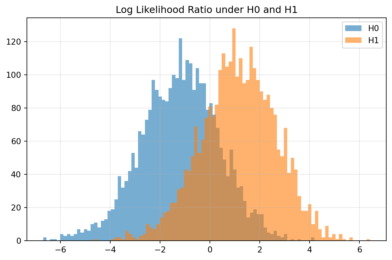

Tradeoff between Type I and Type II errors (power)

rows = []

# jitter everything used for decisions
LLR_H0_j = [jitter(s, 1e-8) for s in LLR_H0]
LLR_H1_j = [jitter(s, 1e-8) for s in LLR_H1]
means_H0_j = [jitter(m, 1e-6) for m in means_H0]
means_H1_j = [jitter(m, 1e-6) for m in means_H1]

alphas = [0.01, 0.05, 0.10, 0.20]

for alpha in alphas:
    # compute cutoffs
    cutoff_LLR = sorted(LLR_H0_j)[int((1 - alpha) * n_simulations)]
    cutoff_mean = sorted(means_H0_j)[int((1 - alpha) * n_simulations)]

    # compute alpha consistently
    alpha_mean = sum(m >= cutoff_mean for m in means_H0_j) / n_simulations
    alpha_LLR = sum(s >= cutoff_LLR for s in LLR_H0_j) / n_simulations

    # compute power consistently
    power_mean = 1 - sum(m < cutoff_mean for m in means_H1_j) / n_simulations
    power_LLR = 1 - sum(s < cutoff_LLR for s in LLR_H1_j) / n_simulations

    rows.append({
        "target_alpha": alpha,
        "alpha_mean": alpha_mean,
        "alpha_LLR": alpha_LLR,
        "power_mean": power_mean,
        "power_LLR": power_LLR
    })

df = pd.DataFrame(rows)

print(df)

   target_alpha  alpha_mean  alpha_LLR  power_mean  power_LLR
0          0.01        0.01       0.01    0.128000   0.237333
1          0.05        0.05       0.05    0.328333   0.465667
2          0.10        0.10       0.10    0.474667   0.594333
3          0.20        0.20       0.20    0.661000   0.761667

Off-ramp: what the Log Likelihood Ratio is

def log_likelihood_ratio(sample):
    total = 0 #initialize total at zero
    for x in sample:
        p1 = probabilities_rigged[x-1]
        p0 = probabilities_fair[x-1]
        total += math.log(p1/p0)
    return total

The function log_likelihood_ratio processes the sample one observation at a time. For each observed value x in the sample:

p1 is the probability of observing x under the alternative hypothesis (rigged d6),
p0 is the probability of observing x under the null hypothesis (fair d6).

The function then compares these two probabilities by forming the ratio p1 / p0, taking the logarithm of this ratio, and adding the result to the running total. Once all observations are processed in this fashion, the function returns the sum of all log-likelihood ratios in the sample.

You can think of each observation as contributing a small piece of evidence:

if p1 > p0, the observation is more likely under the alternative hypothesis, so it contributes a positive amount,
if p1 < p0, the observation is more likely under the null hypothesis, so it contributes a negative amount,
if p1 = p0, the observation is equally likely under both hypotheses, so it contributes nothing (the logarithm of 1 is 0)

The final statistic is the sum of these contributions across all observations.

The Neyman–Pearson lemma shows that, for testing one hypothesis against another, the Log Likelihood Ratio statistic is optimal in the sense that it gives the most powerful test for a given type I error probability level (alpha). It outperforms all other test statistics, including the sample mean.

Full script (all code blocks stacked)



#%% Setup imports and random number generator seed

## First, we need python to import the `random` library so we have access
## to random number generators. We will also set an explicit `seed` for the
## random number generator. Setting a seed guarantees that the generator
## returns the same numbers each time it is invoked, so our results stay
## the same each time we execute this script, as long as we do so in the
## same set sequence.

import random
random.seed(12345)


## Let us start with a simple virtual coin toss.

#%% Coin toss first attempt

coin_1 = random.randint(0, 1)
print(coin_1)


#%% Coin toss another one

coin_2 = random.randint(0, 1)
print(coin_2)


## Our simple coin toss uses the function `randint` from the python library
## `random`. If we open the documentation, we find that `randint(a, b)`
## returns a random integer between `a` and `b`, including both endpoints.
## In our case, we use `randint(0, 1)`, which means the function returns
## either `0` or `1` with equal probability. This gives us a simple way to
## represent the two possible outcomes of a fair coin toss.

#%% Returning a more familiar Heads or Tails

coin = random.randint(0, 1)
if coin == 0:
    coin_face = "Heads"
else:
    coin_face = "Tails"
print(coin_face)


#%% Bestoffive anyone

## For a best-of-five, we will hold the printing until the end, by
## appending each result to a string.
## Strings are collections of characters (for example, words or sentences
## enclosed in quotes such as "Heads" or "Tails" or "This is a string").
## You can concatenate strings by using the operator `+`. For example:
## "Heads" + ", " + "Tails" produces the string "Heads, Tails".
## We will also use the operator `+=`, which means “take the current value
## of the variable and add something to it”. In other words,
## `x += y` is a shorter way of writing `x = x + y`.
## Each time we update our string with `+=`, we are extending it by adding
## new content at the end.

## We will also use a `for` loop, which is a way to instruct python to
## repeat the same block of code several times in sequence.

coin_face_sequence = "" # initialize an empty string

for coin_toss in range(5):
    coin = random.randint(0, 1)
    if coin == 0:
        coin_face_sequence += "Heads, "
    else:
        coin_face_sequence += "Tails, "

print(coin_face_sequence)


#%% Another bestoffive

coin_face_sequence = ""

for coin_toss in range(5):
    coin = random.randint(0, 1)
    if coin == 0:
        coin_face_sequence += "Heads, "
    else:
        coin_face_sequence += "Tails, "

print(coin_face_sequence)


## Wait, that is just the same sequence again!

#%% Another just to be sure

coin_face_sequence = ""

for coin_toss in range(5):
    coin = random.randint(0, 1)
    if coin == 0:
        coin_face_sequence += "Heads, "
    else:
        coin_face_sequence += "Tails, "

print(coin_face_sequence)


## OK, so at least we know it is not always giving us the same sequence.

#%% Offramp random number generator seed

## Let us experiment a bit with the seed, to understand better what it
## does.

random.seed(123)
print("\n random.seed has just been reset")

coin_face_sequence = ""

for coin_toss in range(8):
    coin = random.randint(0, 1)
    if coin == 0:
        coin_face_sequence += "Heads, "
    else:
        coin_face_sequence += "Tails, "

print(coin_face_sequence)


random.seed(123)
print("\n random.seed has just been reset AGAIN")

coin_face_sequence = ""

for coin_toss in range(8):
    coin = random.randint(0, 1)
    if coin == 0:
        coin_face_sequence += "Heads, "
    else:
        coin_face_sequence += "Tails, "

print(coin_face_sequence)


print("\n random.seed has NOT been reset")

coin_face_sequence = ""

for coin_toss in range(8):
    coin = random.randint(0, 1)
    if coin == 0:
        coin_face_sequence += "Heads, "
    else:
        coin_face_sequence += "Tails, "

print(coin_face_sequence)


## The random number generator is deterministic. Once we fix the seed at
## the beginning of a script, the same sequence of values will then always
## be the same, as long as we follow the same sequence of calls.

## Setting a seed ensures **reproducibility of simulation methods**.

## That was probably enough coin tosses for one day. We need to roll dice.

#%% Rolling a d6
## `randint(1, 6)` returns one of the values `1`, `2`, `3`, `4`, `5`, or
## `6`, each with equal probability, simulating a fair six-sided die (also
## known as a **d6**).

roll_d6 = random.randint(1, 6)
print(roll_d6)


#%% Repeated d6 rolls manual observation
## Before moving to repeated rolling, a point of python convention: we
## always start counting at `0`, not at `1`.
## It can be confusing to mix code conventions and plain English, e.g.
## "first" being associated with index `0`. We can use the inelegant but
## hopefully clearer 0-th, 1-th, 2-th in text to indicate python indexing.
## For example,
roll_the_string= "roll"  # a string
print("The 0-th character in the string is:   ", roll_the_string[0])
roll_the_list= ["r", "o", "l", "l"] ## a list of strings
print("The 1-th element in", roll_the_list, "is", roll_the_list[1])
d6_faces= [1, 2, 3, 4, 5, 6] ## a list of integers
print("The 2-th element in", d6_faces, "is", d6_faces[2])


## Rolling a d6, 4 times
roll_0 = random.randint(1, 6)
roll_1 = random.randint(1, 6)
roll_2 = random.randint(1, 6)
roll_3 = random.randint(1, 6)

print(roll_0, roll_1, roll_2, roll_3)

## This code works, but it is repetitive. We will improve this shortly.

#%% Create empty list

results = []
print(results)


#%% Append to a list

roll_0 = random.randint(1, 6)
results.append(roll_0)
print(results)


roll_1 = random.randint(1, 6)
results.append(roll_1)
print(results)


roll_2 = random.randint(1, 6)
results.append(roll_2)
print(results)


roll_3 = random.randint(1, 6)
results.append(roll_3)
print(results)


#%% Inspect sample size length of a list

length_results = len(results)
print("We have completed", length_results, "rolls.")


#%% Inspect values

print("The 0-th roll resulted in a", results[0], ".")
print("The 1-th roll resulted in a", results[1], ".")


#%% Offramp variable semantics
## What happens if we try to modify the 2-th roll?

roll_2 = random.randint(1, 6)
print(roll_2)
results.append(roll_2)
print(results)


## Let's try again, to understand why that did not work.
roll_2 = random.randint(1, 6)
print(roll_2)
results.append(roll_2)
print(results)


## If we were hoping to replace the 2-th (third in natural English
## counting) roll in the sequence, this did not work. There are two issues:

## - `roll_2` makes sense to a human (or an LLM) as referring to the 2-th (third in natural English counting) roll in a sequence, but the machine only does what we ask. A name such as `roll_2` is only a label chosen by the programmer. It suggests an order, but this order is not enforced by the structure of the program, we could equally well call the variable `bob` or `roll55`.
## - we used the `.append` method, which **adds an element at the end of a list**.

## Lists can also be modified element by element. Here is another way to
## roll 4 times

roll_results = ["?", "?", "?", "?"]
print(roll_results)

roll = random.randint(1, 6)
roll_results[0] = roll
print(roll_results)

roll = random.randint(1, 6)
roll_results[1] = roll
print(roll_results)

## I did not enjoy this 1-th roll. It does not count. Try again.

roll = random.randint(1, 6)
roll_results[1] = roll
print(roll_results)

## This 1-th roll does not count either. Try again.

roll = random.randint(1, 6)
roll_results[1] = roll
print(roll_results)

## Much better.

roll = random.randint(1, 6)
roll_results[2] = roll
print(roll_results)

roll = random.randint(1, 6)
roll_results[3] = roll
print(roll_results)


## This approach allows us to:
## - assign values to specific positions,
## - modify values after they have been assigned,
## - treat the list as a fixed structure.

## This also shows the difference between a **cosmetic index** such as
## `roll_2` and a **structural index** such as `roll_results[2]`.
## `roll_results[2]` refers to the 2-th element inside the list
## `roll_results`: it always refers to the same location, and changing it
## modifies the list object itself.

#%% Define function
## At some point, we should try to automate all these d6 rolls. Writing
## functions allows us to reuse the same block of code with different
## inputs, instead of copying it multiple times.

def n_rolls_d6(n):
    results = []
    for i in range(n):
        roll = random.randint(1, 6)
        results.append(roll)
    return results


#%% Generate a small sample

results_small = n_rolls_d6(4)
print(results_small)


#%% Inspect length of small sample

length_small = len(results_small)
print(length_small)


#%% Generate a larger sample

results_large = n_rolls_d6(20)
print(results_large)


#%% Inspect length of large sample

length_large = len(results_large)
print(length_large)


#%% Sort results

sorted_results = sorted(results_large)
print(sorted_results)


#%% Count ones

count_1 = sorted_results.count(1)
print(count_1)


#%% Compare counts

count_1 = sorted_results.count(1)
count_6 = sorted_results.count(6)

print(count_1)
print(count_6)


#%% Count all outcomes

print("Out of", length_large, "rolls, ")
print(results_large)
for value in range(1, 7):
    count = sorted_results.count(value)
    print(value, "was rolled", count, "times.")


#%% Collect counts into a list

## We already counted how many times each value appears. Let us collect
## these counts into a list so that we can manipulate them more easily.

counts = []
for value in range(1, 7):
    count = sorted_results.count(value)
    counts.append(count)

print(counts)


## The sum of counts should be equal to the total number of rolls.

print(sum(counts))
print(length_large)


#%% Labelling the counts explicitly

for value in range(1, 7):
    count = sorted_results.count(value)
    print("Value", value, "appears", count, "times.")

#%% A quick visual comparison

for value in range(1, 7):
    count = sorted_results.count(value)
    bar = "*" * count
    print(value, bar)


## This gives a rough visual comparison of how often each value appears.

#%% A better visualization of counts plotting

import matplotlib.pyplot as plt

results_large = n_rolls_d6(20)

counts_20 = []
for value in range(1, 7):
    counts_20.append(results_large.count(value))

plt.figure()

plt.bar(range(1, 7), counts_20, width=0.6)

plt.title("Counts of d6 rolls (n=20)")
plt.xlabel("Value")
plt.ylabel("Count")

plt.grid(axis="y")
plt.xticks(range(1, 7))

plt.show()
plt.close()


#%% Increasing the sample size

results_200 = n_rolls_d6(200)
sorted_200 = sorted(results_200)
print(results_200)


length_200 = len(results_200)
print("Number of rolls:", length_200)


#%% Visual representation for the larger sample

results_200 = n_rolls_d6(200)

counts_200 = []
for value in range(1, 7):
    counts_200.append(results_200.count(value))

plt.figure()

plt.bar(range(1, 7), counts_200, width=0.6)

plt.title("Counts of d6 rolls (n=200)")
plt.xlabel("Value")
plt.ylabel("Count")

plt.grid(axis="y")
plt.xticks(range(1, 7))

plt.show()
plt.close()


#%% From counts to frequencies
## Counts depend on how many d6 rolls we performed, so instead we focus on
## the **frequency** of each value v, defined as the number of times v
## appears, divided by the total number of rolls. Frequencies take values
## between `0` and `1`, and can be interpreted as empirical probabilities.

print("Sample of 20:")
for value in range(1, 7):
    count = sorted_results.count(value)
    frequency = count / length_large
    print(value, frequency)

print("\nSample of 200:")
for value in range(1, 7):
    count = sorted_200.count(value)
    frequency = count / length_200
    print(value, frequency)



#%% Sidebyside comparison better

# theoretical (fair d6)
theoretical = [1/6 for _ in range(1, 7)]

# empirical n = 20
freq_20 = []
for value in range(1, 7):
    count_20 = sorted_results.count(value)
    freq_20.append(count_20 / length_large)

# empirical n = 200
freq_200 = []
for value in range(1, 7):
    count_200 = sorted_200.count(value)
    freq_200.append(count_200 / length_200)

print("value  prob    n=20         n=200")
for i in range(6): ## i+1 is one face of a d6
    print(
        i+1,
        theoretical[i],
        freq_20[i],
        freq_200[i]
    )


#%% Offramp formatting and padding to create aligned tables

## The following code improves readability of printed tables by aligning
## columns. This is not essential for the main logic, but can be useful for
## presentation.

def pad(text, width=12):
    return text + " " * (width - len(text))

print(
    pad("value")
    + pad("prob")
    + pad("n=20")
    + pad("n=200")
)

for i in range(6): ## i+1 is one face of a d6

    v = str(i + 1)

    t = f"{theoretical[i]:.3f}"
    p20 = f"{freq_20[i]:.3f}"
    p200 = f"{freq_200[i]:.3f}"

    print(
        pad(v)
        + pad(t)
        + pad(p20)
        + pad(p200)
    )


#%% Offramp formatting via a dataframe

## We can avoid manual formatting by using a dataframe.
import pandas as pd

values = list(range(1, 7))

df = pd.DataFrame({
    "value": values,
    "prob": theoretical,
    "n=20": freq_20,
    "n=200": freq_200
})

df = df.set_index("value")
df_rounded = df.round(3)
print(df_rounded)


#%% repeating the experiment with more rolls

## Let us add more samples.
## Note: the following code is very repetitive and not an example of good
## practice. If you find yourself copy-pasting large code blocks, there is
## usually a better way, typically writing a helper function.

results_200_b = n_rolls_d6(200)
sorted_200_b = sorted(results_200_b)
freq_200_b = []

for value in range(1, 7):
    count_200_b = sorted_200_b.count(value)
    freq_200_b.append(count_200_b / len(results_200_b))

results_2000 = n_rolls_d6(2000)
sorted_2000 = sorted(results_2000)
freq_2000 = []

for value in range(1, 7):
    count_2000 = sorted_2000.count(value)
    freq_2000.append(count_2000 / len(results_2000))
    
results_2000_b = n_rolls_d6(2000)
sorted_2000_b = sorted(results_2000_b)
freq_2000_b = []

for value in range(1, 7):
    count_2000_b = sorted_2000_b.count(value)
    freq_2000_b.append(count_2000_b / len(results_2000_b))

results_20000 = n_rolls_d6(20000)
sorted_20000 = sorted(results_20000)
freq_20000 = []

for value in range(1, 7):
    count_20000 = sorted_20000.count(value)
    freq_20000.append(count_20000 / len(results_20000))

results_20000_b = n_rolls_d6(20000)
sorted_20000_b = sorted(results_20000_b)
freq_20000_b = []

for value in range(1, 7):
    count_20000_b = sorted_20000_b.count(value)
    freq_20000_b.append(count_20000_b / len(results_20000_b))
        

df = pd.DataFrame({
    "value": values,
    "prob": theoretical,
    "n=20": freq_20,
    "n=200": freq_200,
    "200_b": freq_200_b,
    "n=2000": freq_2000,
    "2000_b": freq_2000_b,
    "n=20000": freq_20000,
    "20000_b": freq_20000_b,
})
df = df.set_index("value")
df_rounded = df.round(4)
print(df_rounded)



#%% repeating the experiment with more rolls compact code version
## A more compact, less error-prone version of the same code:

values = list(range(1, 7))
# theoretical (fair d6)
theoretical = [1/6 for _ in range(1, 7)]

def compute_frequencies(n):
    results = n_rolls_d6(n)
    frequencies = []
    for value in range(1, 7):
        count = results.count(value)
        frequencies.append(count / len(results))
    return frequencies

df_series={
    "value": values,
    "prob": theoretical,}
    
series_names_list=[]
for n in [20,200,200,2000,2000,20000,20000]:
    series_name="n="+str(n) ## string concatenation
    if series_name in series_names_list:
        series_name+="_"  ## if two samples have the same size
    series_names_list.append(series_name)
    df_series[series_name]=compute_frequencies(n)
df = pd.DataFrame(df_series)
df = df.set_index("value")
df_rounded = df.round(4)

print(df_rounded)


#%% Visualizations using frequencies and sample size

## The previous visualizations used counts. Let us now visualize
## **frequencies**.

plt.figure()

plt.bar(range(1, 7), freq_200, width=0.6)

plt.axhline(1/6, color="black", linestyle="--")  # theoretical frequency

plt.title("Frequencies of d6 rolls (n=200)")
plt.xlabel("Value")
plt.ylabel("Frequency")


plt.xticks(range(1, 7))

# y tickmarks at multiples of 1/24
plt.yticks([i/24 for i in range(25)])  ## list comprehension

## Restrict span of the vertical axis
max_height = max(freq_200)
y_max = 1.15 * max_height

plt.ylim(0, y_max)

plt.grid(axis="y")

plt.show()
plt.close()


## Again, for the larger sample.


plt.figure()

plt.bar(range(1, 7), freq_20000, width=0.6)

plt.axhline(1/6, color="black", linestyle="--")  # theoretical frequency

plt.title("Frequencies of d6 rolls (n=20000)")
plt.xlabel("Value")
plt.ylabel("Frequency")

plt.grid(axis="y")
plt.xticks(range(1, 7))

# y tickmarks at multiples of 1/24
plt.yticks([i/24 for i in range(25)])

## Restrict span of the vertical axis
max_height = max(freq_20000)
y_max = 1.15 * max_height

plt.ylim(0, y_max)
plt.show()
plt.close()


## Across repeated samples:

## - Frequencies vary from sample to sample.
## - For large samples, frequencies are close to the theoretical probability $\frac{1}{6}$.
## - Sample frequencies converge toward their theoretical probability as the sample size grows, this is an instance of the **law of large numbers**.

#%% Descriptive statistics
## We now move from looking at raw data and frequencies to **summarizing
## data**. Some vocabulary:

## A **random variable** is a numerical quantity generated by a random
## process (for example, one roll of a d6).

## A **realization** or **observation**  is a value that the random
## variable actually takes when executing the random process (for example,
## observing a `4` upon rolling a d6).

## A **sample** or **data series**  is a finite list of realizations. The
## number of observations is the **sample size**.

## A **statistic** is a number computed from a data series to quantify one
## of its features.

## We will construct a data series where each observation is the sum of
## four d6 rolls (4d6).

import random

def roll_4d6():
    total = 0
    for i in range(4):
        total += random.randint(1, 6)
    return total

def generate_4d6_series(n_observations):
    results = []
    for i in range(n_observations):
        results.append(roll_4d6())
    return results


## Note: The function `generate_4d6_series` repeatedly calls the function
## `roll_4d6`.

n_observations_4d6 = 800

rolls_4d6 = generate_4d6_series(n_observations_4d6)

print(rolls_4d6[:10])

## It's always a good idea to print a small amount of your dataset and/or
## visually inspect it.
## It's also a good idea to try to visualize your variables, typically with
## histograms or summary tables.



frequencies_4d6 = [
    rolls_4d6.count(total)
    for total in range(4, 25)
]

plt.bar(range(4, 25), frequencies_4d6)
plt.xlabel("Sum of four d6 rolls")
plt.ylabel("Frequency")
plt.xticks(range(4, 25))
plt.show()


#%% Mean

mean_4d6 = sum(rolls_4d6) / n_observations_4d6
print(mean_4d6)




#%% Minimum and maximum

print(min(rolls_4d6), max(rolls_4d6))




#%% Median

sorted_4d6 = sorted(rolls_4d6)

median_4d6 = sorted_4d6[n_observations_4d6 // 2]

print(median_4d6)




#%% Quantiles and quartiles

q25_4d6 = sorted_4d6[n_observations_4d6 // 4]
q50_4d6 = sorted_4d6[n_observations_4d6 // 2]
q75_4d6 = sorted_4d6[(3 * n_observations_4d6) // 4]

print(q25_4d6, q50_4d6, q75_4d6)

iqr_4d6 = q75_4d6 - q25_4d6
print(iqr_4d6)




#%% Variance and standard deviation

sq_diffs_4d6 = []

for value in rolls_4d6:
    diff = value - mean_4d6
    sq_diffs_4d6.append(diff**2)

variance_4d6 = sum(sq_diffs_4d6) / (n_observations_4d6-1)
## we divide by (n-1) because <stats reasons>, 
## see a stats textbook on "sample variance"
std_4d6 = variance_4d6 ** 0.5

print(variance_4d6)
print(std_4d6)





#%% Summary and describe

## We have now introduced several statistics used to describe a data
## series.
## - A **measure of location** summarizes central tendency (mean, median, mode)
## - A **measure of dispersion** summarizes variability (variance, standard deviation, interquartile range)

## These statistics can be computed manually, as we have done so far. They
## can also be obtained automatically using the `.describe()` method from
## the `pandas` library, which returns a standard set of summary statistics
## for each variable in a dataframe.

import pandas as pd

df_4d6 = pd.DataFrame({
    "rolls_4d6": rolls_4d6
})

print("d6 summary:")
print(df_4d6.describe())


#%% Rigged d6 vs fair d6 construction

## We now move to hypothesis testing. So far, we have described data
## generated by a known data generating process. We now reverse the
## perspective: we observe data and try to infer the data generating
## process that produced it.

## First, we need to define what a rigged d6 is and implement it in code.

## We will construct both a fair d6 and a rigged d6 using the same
## interval-based method, making their probability distributions easy to
## compare.

import random
import matplotlib.pyplot as plt
import pandas as pd

random.seed(1236)

interval_widths_fair = [12, 12, 12, 12, 12, 12]
interval_widths_rigged = [10, 8, 12, 12, 16, 14]

assert sum(interval_widths_fair) == 72
assert sum(interval_widths_rigged) == 72

thresholds_fair = []
running_total = 0

for interval_width in interval_widths_fair:
    running_total += interval_width
    thresholds_fair.append(running_total)

thresholds_rigged = []
running_total = 0

for interval_width in interval_widths_rigged:
    running_total += interval_width
    thresholds_rigged.append(running_total)

probabilities_fair = []

for interval_width in interval_widths_fair:
    probabilities_fair.append(interval_width / 72)

probabilities_rigged = []

for interval_width in interval_widths_rigged:
    probabilities_rigged.append(interval_width / 72)

def roll_fair_d6():

    draw = random.randint(1, 72)

    for face, threshold in enumerate(thresholds_fair, start=1):
        if draw <= threshold:
            return face

def roll_rigged_d6():

    draw = random.randint(1, 72)

    for face, threshold in enumerate(thresholds_rigged, start=1):
        if draw <= threshold:
            return face


#%% Rigged d6 vs fair d6 visualizing the mapping

import matplotlib.pyplot as plt

plt.figure(figsize=(10, 3))

plt.hlines(2, 1, 72)

for threshold in thresholds_fair:
    plt.vlines(threshold, 2, 2.6, color="blue")

for threshold in thresholds_rigged:
    plt.vlines(threshold, 1.4, 2, color="red")

all_ticks = sorted(set([1] + thresholds_fair + thresholds_rigged))

start = 1

for face, interval_width in enumerate(interval_widths_fair, start=1):
    midpoint = start + (interval_width - 1) / 2
    plt.text(midpoint, 2.2, str(face), color="blue", ha="center", fontsize=12)
    start += interval_width

start = 1

for face, interval_width in enumerate(interval_widths_rigged, start=1):
    midpoint = start + (interval_width - 1) / 2
    plt.text(midpoint, 1.6, str(face), color="red", ha="center", fontsize=12)
    start += interval_width

plt.xlim(1, 72)
plt.ylim(1.4, 2.6)

plt.xticks(all_ticks)
plt.yticks([])

ax = plt.gca()
ax_top = ax.secondary_xaxis("top")

ax_top.set_xticks(all_ticks)
ax_top.set_xticklabels(all_ticks)

plt.grid(axis="x", alpha=0.3)

plt.title("Mapping from [1,72] to d6 outcomes")
plt.xlabel("Integer draw")

plt.show()


## Blue labels correspond to the fair d6 mapping.

## Red labels correspond to the rigged d6 mapping.

## - fair d6: each face receives 12 integers and therefore occurs with probability \(12/72 = 1/6\)
## - rigged d6: each face receives a different number of integers and therefore occurs with a different probability

## The probability distributions implied by the two data generating
## processes are:

df_probabilities = pd.DataFrame({
    "face": [1, 2, 3, 4, 5, 6],
    "probabilities_fair": probabilities_fair,
    "probabilities_rigged": probabilities_rigged
})

print(df_probabilities.round(3))


#%% Empirical comparison and varying the sample size

## We now generate samples from each d6 and compare their empirical
## frequencies with the corresponding theoretical probabilities.

sample_sizes = [20, 200, 2000, 20000]

results_all = []
max_height = 0

for sample_size in sample_sizes:

    sample_fair = []

    for roll_number in range(sample_size):
        sample_fair.append(roll_fair_d6())

    sample_rigged = []

    for roll_number in range(sample_size):
        sample_rigged.append(roll_rigged_d6())

    freqs_fair = []

    for face in range(1, 7):
        freqs_fair.append(
            sample_fair.count(face) / sample_size
        )

    freqs_rigged = []

    for face in range(1, 7):
        freqs_rigged.append(
            sample_rigged.count(face) / sample_size
        )

    results_all.append(
        (
            sample_size,
            freqs_fair,
            freqs_rigged
        )
    )

    max_height = max(
        max_height,
        max(freqs_fair),
        max(freqs_rigged)
    )

y_max = 1.15 * max_height

step = 1 / 36
yticks = []
current = 0

while current <= y_max:
    yticks.append(current)
    current += step

fig, axes = plt.subplots(4, 2, figsize=(8, 16))

for row, (sample_size, freqs_fair, freqs_rigged) in enumerate(results_all):

    axes[row, 0].bar(range(1, 7), freqs_fair, color="blue")

    for face, probability in enumerate(probabilities_fair, start=1):
        axes[row, 0].hlines(
            probability,
            face - 0.3,
            face + 0.3,
            linestyles="--",
            color="black"
        )

    axes[row, 0].set_title(f"Fair d6 (n={sample_size})")
    axes[row, 0].grid(axis="y", alpha=0.3)

    axes[row, 1].bar(range(1, 7), freqs_rigged, color="red")

    for face, probability in enumerate(probabilities_rigged, start=1):
        axes[row, 1].hlines(
            probability,
            face - 0.3,
            face + 0.3,
            linestyles="--",
            color="black"
        )

    axes[row, 1].set_title(f"Rigged d6 (n={sample_size})")
    axes[row, 1].grid(axis="y", alpha=0.3)

    for col in [0, 1]:
        axes[row, col].set_ylim(0, y_max)
        axes[row, col].set_yticks(yticks)

plt.tight_layout()
plt.show()


## Across repeated samples:

## - Frequencies vary from sample to sample.
## - For large samples, frequencies are close to the theoretical probability for each face.

## Differences across samples are an example of **sampling variation**.

## For large samples, empirical frequencies tend to become close to the
## corresponding theoretical probabilities. This is another illustration of
## the **Law of Large Numbers**.

#%% Testing whether a given d6 is fair

## We now move from describing samples to making decisions from them.
## Suppose we are given a sample of n=50 rolls from a d6 with unknown type.
## A natural question is: *Based on the evidence, is this d6 fair, or is it
## rigged?*

## The code below recreates this uncertainty by randomly deciding whether
## each sample comes from the fair d6 or the rigged d6. You can run it
## multiple times to generate a new collection of unknown samples.

sample_size = 50
prob_rigged = 0.48

fig, axes = plt.subplots(3, 2, figsize=(8, 12))

fair_indices = []  # store outcomes for printing later
rigged_indices = []  # store outcomes for printing later

for i in range(6): ## draw 6 samples (6 simulations)

    is_rigged = random.random() < prob_rigged

    if is_rigged:

        sample_unknown = []

        for roll_number in range(sample_size):
            sample_unknown.append(roll_rigged_d6())

        rigged_indices.append(i)

    else:

        sample_unknown = []

        for roll_number in range(sample_size):
            sample_unknown.append(roll_fair_d6())

        fair_indices.append(i)

    freqs_unknown = []

    for face in range(1, 7):
        freqs_unknown.append(
            sample_unknown.count(face) / sample_size
        )

    row = i // 2
    col = i % 2
    ax = axes[row, col]

    ax.bar(range(1, 7), freqs_unknown, width=0.6, color="gray", alpha=0.5)

    for x, y in enumerate(probabilities_fair, start=1):
        ax.hlines(y, x-0.3, x+0.3, linestyles="--", color="blue")

    for x, y in enumerate(probabilities_rigged, start=1):
        ax.hlines(y, x-0.3, x+0.3, linestyles=":", color="red")

    ax.set_title(f"Unknown_{i} d6 (n={sample_size})")
    ax.set_xlabel("Value")
    ax.set_ylabel("Frequency")

    ax.grid(axis="y")
    ax.set_xticks(range(1, 7))

    # y tickmarks
    ax.set_yticks([i/36 for i in range(37)])

    # restrict vertical axis
    max_height = max(freqs_unknown)
    y_max = 1.2 * max_height
    ax.set_ylim(0, y_max)

plt.tight_layout()
plt.show()

# print results after all plots
print("The fair d6 types were", fair_indices, ". The rigged d6 types were", rigged_indices)


## We know that the histogram from the rigged d6 is  “lopsided”, but how
## lopsided is *too* lopsided? We need a systematic way to decide. Staring
## at histograms and going with visual intuition is not transparent or
## reproducible. Instead, we introduce two tools:

## - a **test statistic**: a number computed from the sample
## - a **decision rule**: a rule telling us when that number is “too extreme”

## A test statistic summarizes the information contained in the sample (the
## six empirical frequencies) into a single number. We should typically get
## higher sample means from the rigged d6, so we will use the sample mean
## as a test statistic to detect a rigged d6. The sample mean is not the
## best available test statistic, we will return to that point later.

values = [1,2,3,4,5,6]

expected_fair = sum(v*p for v,p in zip(values,probabilities_fair))
expected_rigged = sum(v*p for v,p in zip(values,probabilities_rigged))

print(f"Expected sample mean (fair d6): {expected_fair:.3f}")
print(f"Expected sample mean (rigged d6): {expected_rigged:.3f}")


import matplotlib.pyplot as plt

sample_size = 50
n_simulations = 400

means_fair = []
means_rigged = []

for _ in range(n_simulations):
    sample_fair = [roll_fair_d6() for _ in range(sample_size)]
    sample_rigged = [roll_rigged_d6() for _ in range(sample_size)]
    
    means_fair.append(sum(sample_fair) / sample_size)
    means_rigged.append(sum(sample_rigged) / sample_size)

# build discrete frequencies
x_vals = sorted(set(means_fair + means_rigged))

freqs_fair = []
freqs_rigged = []

for x in x_vals:
    freqs_fair.append(means_fair.count(x) / n_simulations)
    freqs_rigged.append(means_rigged.count(x) / n_simulations)

bar_width = 1 / sample_size

plt.figure(figsize=(8,5))

plt.bar(x_vals, freqs_fair, width=bar_width, alpha=0.6, color="darkblue", label="fair d6")
plt.bar(x_vals, freqs_rigged, width=bar_width, alpha=0.6, color="darkred", label="rigged d6")

plt.axvline(expected_fair, color="black", linestyle="--")

plt.xlabel(f"sample mean (n={sample_size})")
plt.ylabel("frequency")
plt.title(f"Sample mean (n={sample_size}), across {n_simulations} simulations")
plt.legend()

plt.grid(alpha=0.3)

plt.show()


## The two distributions are centered at different values: high sample
## means are more likely to happen with a rigged d6 than with a fair d6.
## However, the two distributions overlap: some rigged d6 samples have a
## lower sample mean than some fair d6 samples. So the sample mean is an
## imperfect statistic and we will never be able to guarantee that we can
## detect a rigged d6 using only a sample of 50 rolls. In general,
## hypothesis testing does not produce definitive answers, instead it aims
## to quantify uncertainty.

#%% Hypotheses decision rule type I error and type II error

## A statistical hypothesis test is a procedure to formally decide whether
## there is enough information in the data available to reject a particular
## statement known as the **null hypothesis**. In our application,

## - null hypothesis $H_0$: the d6 is fair
## - alternative hypothesis $H_{1}$: the d6 is rigged

## **Decision rule**: If the null hypothesis is correct, the d6 is fair,
## and the sample mean should be close to 3.5. If the sample mean is
## sufficiently far from 3.5, we reject the null hypothesis. The challenge
## is to formally and transparently decide on what "close to" and
## "sufficiently far from" mean for our application.

## Any decision rule gives rise to two types of errors:
## A **type I error** (incorrectly reject) corresponds to rejecting $H_0$
## when the d6 is in fact fair.
## A **type II error** (failure to correctly reject) corresponds to failing
## to reject $H_0$ when the d6 is in fact rigged.

## Note that the statistical hypothesis test framework embeds an asymmetry:
## we never accept the null hypothesis, we simply reject or fail to reject
## it. See <https://decodingstatistics.substack.com/p/why-statisticians-
## say-fail-to-reject-instead-of-accept-the-null>.


#%% Distribution of the sample mean under H0

sample_size = 50
n_simulations = 3000

means_H0 = [
    sum(roll_fair_d6() for _ in range(sample_size))/sample_size
    for _ in range(n_simulations)
]

x_vals = sorted(set(means_H0))
freqs = [means_H0.count(x)/n_simulations for x in x_vals]

bar_width = 1/sample_size

plt.figure(figsize=(8,5))
plt.bar(x_vals, freqs, width=bar_width, color="blue")

plt.axvline(expected_fair, linestyle="--")
plt.title("Sample mean under H0")
plt.grid(alpha=0.3)
plt.show()



#%% Decision rule and pvalues

## In hypothesis testing, we first choose a target frequency of Type I
## errors.

## We then reject the null hypothesis for **sufficiently extreme values of
## the test statistic**.

alpha = 0.10

def jitter(x, scale):
    return x + random.uniform(-scale, scale)

means_H0_j = [jitter(m, 1e-6) for m in means_H0]
cutoff_means_H0_j_10pct = sorted(means_H0_j)[int((1-alpha) * n_simulations)]

print(f"Decision rule: reject H0 if sample mean ≥ {cutoff_means_H0_j_10pct:.3f}")


## The same decision rule can be expressed using **p-values**: for a
## realized value of the test statistic T, the p-value of T is the
## probability (under $H_0$) of observing a value at least as extreme as T.
## Small p-values correspond to realizations which are unlikely under
## $H_0$, large p-values correspond to realizations which are likely under
## $H_0$.

## > The realized sample mean T is in the top 10% of possible realizations
## under $H_0$.

## is equivalent to

## > The realized sample mean T has a p-value (under $H_0$) of 0.1 or less.


#%% Visualizing the rejection region

x_fail = []
y_fail = []
x_reject = []
y_reject = []

for x, y in zip(x_vals, freqs):
    if x < cutoff_means_H0_j_10pct:
        x_fail.append(x)
        y_fail.append(y)
    else:
        x_reject.append(x)
        y_reject.append(y)

plt.figure(figsize=(8,5))
plt.bar(x_fail, y_fail, width=bar_width, color="blue")
plt.bar(x_reject, y_reject, width=bar_width, color="red")

plt.axvline(cutoff_means_H0_j_10pct, linestyle=":", label="cutoff (90th pctile)", color="black")

plt.title("Decision rule: reject iff sample mean is in the top 10%")
plt.xlabel(f"sample mean (n={sample_size})")
plt.ylabel("frequency")

plt.legend()
plt.grid(alpha=0.3)
plt.show()


## Blue values correspond to realizations for which we **fail to reject
## $H_0$**.
## Red values correspond to realizations for which we **reject $H_0$**.

#%% Simulating repeated tests

## In each simulation, a hypothetical d6-making machine produces a d6,
## which is:
## - a fair d6 with probability `prob_fair`
## - a rigged d6 with probability `prob_rigged`

## 1. the d6 inspector receives the newly-produced d6
## 2. rolls it `sample_size` times
## 3. computes the sample mean
## 4. compares it to the cutoff (90th percentile of sample mean)
## 5. rejects $H_0$ iff the sample mean exceeds the cutoff

## We could equivalently reformulate the inspector's decision in terms of
## p-values:
## 4'. computes the p-value of the sample mean
## 5'. rejects $H_0$ iff the p-value is 0.1 or less

random.seed(999)

min_trials = 20
max_trials = 60
prob_rigged = 0.30
prob_fair = 1 - prob_rigged

def compute_p_value(stat, reference):
    return sum(x >= stat for x in reference) / len(reference)

print(f"Decision rule: reject H0 iff the mean exceeds {cutoff_means_H0_j_10pct:.3f}")

examples = {
    "Type I": None,
    "Type II": None,
    "correct_reject": None,
    "correct_fail": None
}

t = 0

while True:

    is_rigged = random.random() < prob_rigged
    generator = roll_rigged_d6 if is_rigged else roll_fair_d6

    sample = [generator() for _ in range(sample_size)]
    m = sum(sample) / sample_size
    m_j = jitter(m, 1e-6)

    p_value = compute_p_value(m, means_H0)
    reject = m_j >= cutoff_means_H0_j_10pct

    if is_rigged and reject:
        outcome = "correctly reject H0 while d6 is rigged"
        key = "correct_reject"
    elif is_rigged:
        outcome = "Type II; fail to reject H0 while d6 is rigged"
        key = "Type II"
    elif reject:
        outcome = "Type I; incorrectly reject H0 while d6 is fair"
        key = "Type I"
    else:
        outcome = "correctly fail to reject H0 while d6 is fair"
        key = "correct_fail"

    # store first occurrence
    if examples[key] is None:
        examples[key] = {
            "trial": t,
            "mean": m,
            "p": p_value,
            "group": "reject" if key in ["Type I", "correct_reject"] else "fail",
            "is_rigged": is_rigged,
            "outcome": outcome
        }

    print(f"Trial {t:02d} | {'rigged' if is_rigged else 'fair':6s} | mean={m_j:.3f} | p-value={p_value:.3f} | {outcome}")

    t += 1
    # stopping conditions
    all_types_found = all(v is not None for v in examples.values())

    if (t >= min_trials and all_types_found) or t >= max_trials:
        break


## We now place one example of each outcome on the rejection-region figure.

plt.figure(figsize=(8,5))

plt.bar(x_fail, y_fail, width=bar_width, color="blue")
plt.bar(x_reject, y_reject, width=bar_width, color="red")

plt.axvline(cutoff_means_H0_j_10pct, linestyle=":", label="cutoff (90th pctile)")

# simple color map (local, readable)
color_map = {
    "Type I": "black",
    "Type II": "beige",
    "correct_reject": "purple",
    "correct_fail": "pink"
}

# manual y-placement: different across AND within groups
y_positions = {
    "Type I": 0.95,
    "correct_reject": 0.87,
    "Type II": 0.07,
    "correct_fail": 0.15
}

# manual y-align: different in reject
y_align = {
    "Type I": "left",
    "correct_reject": "left",
    "Type II": "center",
    "correct_fail": "center"
}

# plotting
for key, value in examples.items():
    if value is None:
        continue

    x_val = value["mean"]
    trial_id = value["trial"]
    p_val = value["p"]

    color = color_map[key]
    y_text = max(freqs) * y_positions[key]

    # line ends just below text
    y_line = y_text * 0.97

    ha = y_align[key]

    # draw truncated line
    plt.vlines(x_val, 0, y_line, color=color)

    # label close to line (not floating too high)
    plt.text(
        x_val,
        y_text,
        f"T{trial_id:02d} p={p_val:.3f}",
        ha=ha,
        color=color
    )

plt.title("Rejection region with selected trials")
plt.xlabel(f"sample mean (n={sample_size})")
plt.ylabel("frequency")

plt.grid(alpha=0.3)
plt.show()

print("Trials displayed on the figure:")
for key, value in examples.items():
    print(f'T{value["trial"]:02d} | {"rigged" if value["is_rigged"] else "fair":6s} | mean={value["mean"]:.3f} | p-value={value["p"]:.3f} | {key}')


## Each point illustrates:

## - its position relative to the cutoff
## - the corresponding p-value
## - the resulting decision
## - whether that decision is correct or an error



#%% Type II error and power

means_H1 = [
    sum(roll_rigged_d6() for _ in range(sample_size))/sample_size
    for _ in range(n_simulations)
]

rows = []

# jitter everything used for decisions
means_H0_j = [jitter(m, 1e-6) for m in means_H0]
means_H1_j = [jitter(m, 1e-6) for m in means_H1]

alphas = [0.01, 0.05, 0.10, 0.20]

for alpha in alphas:
    # compute cutoffs
    cutoff_mean = sorted(means_H0_j)[int((1 - alpha) * n_simulations)]

    # compute empirical alpha
    alpha_mean = sum(m >= cutoff_mean for m in means_H0_j) / n_simulations

    # compute power
    power_mean = 1 - sum(m < cutoff_mean for m in means_H1_j) / n_simulations

    rows.append({
        "target_alpha": alpha,
        "alpha_mean": alpha_mean,
        "power_mean": power_mean,
    })

df = pd.DataFrame(rows)

print(df)




#%% VARIANT Increasing sample size

## Increasing the sample size reduces noise in the statistic and in turn
## means more power for a given level of type I error.

alpha = 0.10

power_means_H0_j_10pct= 1 - sum(m < cutoff_means_H0_j_10pct for m in means_H1_j) / n_simulations

sample_size_v = 100

means_H0_v = [
    sum(roll_fair_d6() for _ in range(sample_size_v))/sample_size_v
    for _ in range(n_simulations)
]

means_H1_v = [
    sum(roll_rigged_d6() for _ in range(sample_size_v))/sample_size_v
    for _ in range(n_simulations)
]

cutoff_v = sorted(jitter(m,1e-6) for m in means_H0_v)[int((1-alpha)*n_simulations)]
power_v = 1 - sum(jitter(m,1e-6) < cutoff_v for m in means_H1_v)/n_simulations

print(f"Sample size {sample_size}: cutoff={cutoff_means_H0_j_10pct:.3f}, power={power_means_H0_j_10pct:.3f}")
print(f"Sample size {sample_size_v}: cutoff={cutoff_v:.3f}, power={power_v:.3f}")




#%% VARIANT Increasing severity of rigging
alpha = 0.10

interval_widths_rigged_severe = [8, 8, 12, 12, 16, 16]

thresholds_rigged_severe = []
running_total = 0

for interval_width in interval_widths_rigged_severe:
    running_total += interval_width
    thresholds_rigged_severe.append(running_total)

def roll_rigged_severe():

    draw = random.randint(1, 72)

    for face, threshold in enumerate(
        thresholds_rigged_severe,
        start=1
    ):
        if draw <= threshold:
            return face

means_H1_severe = [
    sum(
        roll_rigged_severe()
        for _ in range(sample_size)
    ) / sample_size
    for _ in range(n_simulations)
]

power_severe = (
    1
    - sum(
        jitter(m, 1e-6) < cutoff_means_H0_j_10pct
        for m in means_H1_severe
    )
    / n_simulations
)

print(f"Baseline rigging: cutoff={cutoff_means_H0_j_10pct:.3f}, power={power_means_H0_j_10pct:.3f}")
print(f"More severe rigging: cutoff={cutoff_means_H0_j_10pct:.3f}, power={power_severe:.3f}")

## Note that the cutoff is determined under $H_0$, so the decision rule
## itself (the cutoff) does not depend on how severely rigged the d6 is.
## However, a more severely rigged d6 is easier to detect.

#%% VARIANT A better test statistic Log Likelihood Ratio

## We now construct a better test statistic: the sum of log likelihood
## ratios. The interpretation of this statistic is in a dedicated "off-
## ramp" section. For now, we will just see that this test statistic can be
## used to detect the rigged d6 and that it is better than the sample mean
## in the sense of giving more power (fewer type II errors) for the same
## sample size and the same amount of type I errors.


import math

def log_likelihood_ratio(sample):
    total = 0
    for x in sample:
        p1 = probabilities_rigged[x-1]
        p0 = probabilities_fair[x-1]
        total += math.log(p1/p0)
    return total


LLR_H0=[]
LLR_H1=[]
LLR_H1=[]
for i_simulation in range(n_simulations):
    sample_H0 = [roll_fair_d6() for i_roll in range(sample_size)]
    sample_H1 = [roll_rigged_d6() for i_roll in range(sample_size)]
    
    LLR_H0.append(log_likelihood_ratio(sample_H0))
    LLR_H1.append(log_likelihood_ratio(sample_H1))

plt.figure(figsize=(8,5))
plt.hist(LLR_H0, bins=80, alpha=0.6, label="H0")
plt.hist(LLR_H1, bins=80, alpha=0.6, label="H1")

plt.legend()
plt.title("Log Likelihood Ratio under H0 and H1")
plt.grid(alpha=0.3)
plt.show()


#%% Tradeoff between Type I and Type II errors power


rows = []

# jitter everything used for decisions
LLR_H0_j = [jitter(s, 1e-8) for s in LLR_H0]
LLR_H1_j = [jitter(s, 1e-8) for s in LLR_H1]
means_H0_j = [jitter(m, 1e-6) for m in means_H0]
means_H1_j = [jitter(m, 1e-6) for m in means_H1]

alphas = [0.01, 0.05, 0.10, 0.20]

for alpha in alphas:
    # compute cutoffs
    cutoff_LLR = sorted(LLR_H0_j)[int((1 - alpha) * n_simulations)]
    cutoff_mean = sorted(means_H0_j)[int((1 - alpha) * n_simulations)]

    # compute alpha consistently
    alpha_mean = sum(m >= cutoff_mean for m in means_H0_j) / n_simulations
    alpha_LLR = sum(s >= cutoff_LLR for s in LLR_H0_j) / n_simulations

    # compute power consistently
    power_mean = 1 - sum(m < cutoff_mean for m in means_H1_j) / n_simulations
    power_LLR = 1 - sum(s < cutoff_LLR for s in LLR_H1_j) / n_simulations

    rows.append({
        "target_alpha": alpha,
        "alpha_mean": alpha_mean,
        "alpha_LLR": alpha_LLR,
        "power_mean": power_mean,
        "power_LLR": power_LLR
    })

df = pd.DataFrame(rows)

print(df)



#%% Offramp what the Log Likelihood Ratio is
def log_likelihood_ratio(sample):
    total = 0 #initialize total at zero
    for x in sample:
        p1 = probabilities_rigged[x-1]
        p0 = probabilities_fair[x-1]
        total += math.log(p1/p0)
    return total

## The function `log_likelihood_ratio` processes the sample one observation
## at a time. For each observed value `x` in the sample:

## - p1 is the probability of observing x under the alternative hypothesis (rigged d6),
## - p0 is the probability of observing x under the null hypothesis (fair d6).

## The function then compares these two probabilities by forming the ratio
## p1 / p0, taking the logarithm of this ratio, and adding the result to
## the running total. Once all observations are processed in this fashion,
## the function returns the sum of all log-likelihood ratios in the sample.

## You can think of each observation as contributing a small piece of
## evidence:

## - if p1 > p0, the observation is more likely under the alternative hypothesis, so it contributes a positive amount,
## - if p1 < p0, the observation is more likely under the null hypothesis, so it contributes a negative amount,
## - if p1 = p0, the observation is equally likely under both hypotheses, so it contributes nothing (the logarithm of 1 is 0)

## The final statistic is the sum of these contributions across all
## observations.

## The **Neyman–Pearson lemma** shows that, for testing one hypothesis
## against another, the Log Likelihood Ratio statistic is optimal in the
## sense that it gives the most powerful test for a given type I error
## probability level (alpha). It outperforms all other test statistics,
## including the sample mean.